Single Variable Calculus

Dive into Deep Learning · §24.1

The local linear model behind every optimizer
the derivative · gradient descent · curvature · Taylor · corners.

Which way is downhill?

Motivation

Training stacks every weight into one vector \mathbf{w} and minimizes a loss L(\mathbf{w}) too tangled to solve outright. So we step downhill instead.

Freeze every weight but one and the loss becomes a curve f(x) in a single variable. The whole section answers one question about it:

Which way is downhill, and by how much? The derivative answers both at once.

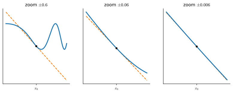
Zoom in on a smooth curve and it flattens onto a line, the tangent at the base point.

The derivative

zooming in, secants, and the tangent slope

Every smooth curve is a line, up close

The derivative

Zoom in on any smooth function and the wiggles flatten until the graph is indistinguishable from a straight line, the tangent, whose slope is all that is left to pin down.

From secant to tangent

The derivative

The difference quotient is the slope of the secant through two nearby points:

\frac{f(x+\epsilon) - f(x)}{\epsilon}.

As \epsilon \to 0 the second point slides in and the secant rotates into the tangent, whose limiting slope is the derivative f'(x).

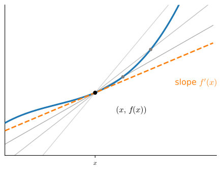
As \epsilon \to 0 the secant through (x,f(x)) and (x+\epsilon,f(x+\epsilon)) rotates into the tangent, whose slope is f'(x).

Watch the slope settle

The derivative

The secant slope of f(x) = x^2 + 1701(x-4)^3 at x=4 marches toward 8 as \epsilon shrinks:

# Define our function
def f(x):
    return x**2 + 1701*(x-4)**3

# Slope of the secant through x=4, for shrinking epsilon
for epsilon in [0.1, 0.001, 0.0001, 0.00001]:
    print(f'epsilon = {epsilon:.5f} -> {(f(4+epsilon) - f(4)) / epsilon:.5f}')

epsilon = 0.10000 -> 25.11000
epsilon = 0.00100 -> 8.00270
epsilon = 0.00010 -> 8.00012
epsilon = 0.00001 -> 8.00001

The table only creeps; autograd returns it exactly, no \epsilon:

autograd: f'(4) = 8.0

The small-change identity

The derivative

Rearranging the limit gives the small-change identity:

f(x+\epsilon) \approx f(x) + \epsilon\,f'(x).

Nudge the input by \epsilon, the output moves by \epsilon times the derivative. The derivative is the exchange rate between an input change and the output change it buys, and the differentiation rules, gradient descent, and Taylor series are all applications of this one line.

Linear approximation & descent

the tangent line becomes a step downhill

The tangent line is the best local model

Optimization

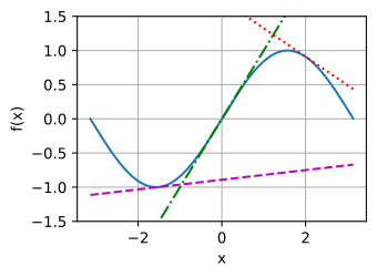
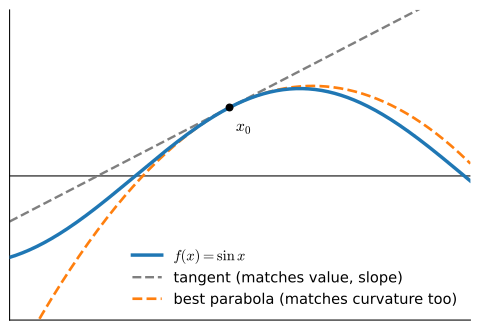
Read as a function of the displacement, f(x+\epsilon) \approx f(x) + \epsilon f'(x) is the tangent line at x, the best straight-line model of f nearby.

Drawn at three points of \sin (using \tfrac{d}{dx}\sin = \cos), each line hugs the curve in a neighborhood and peels away beyond it.

The gradient-descent step

Optimization

Now we choose the step. Take \epsilon = -\eta\,f'(x) with step size \eta > 0: moving against the slope makes the model drop by

\approx \eta\,[f'(x)]^2 \ge 0.

Whatever the sign of f', stepping against it lowers f, by an amount proportional to the slope squared. Iterating is gradient descent, x_{t+1} = x_t - \eta f'(x_t).

The descent lemma, in one picture

Optimization

If the slope is L-Lipschitz, the curvature erects a quadratic ceiling f(x) + f'(x)s + \tfrac{L}{2}s^2 that touches the graph at the base point.

Stepping to the ceiling’s minimizer (the gradient step with \eta = 1/L) drops f by at least \tfrac{1}{2L}[f'(x)]^2:

f\!\left(x - \eta f'(x)\right) \le f(x) - \eta\!\left(1 - \tfrac{L\eta}{2}\right)[f'(x)]^2.

A strict decrease for every 0 < \eta < 2/L.

Five step sizes, five regimes

Optimization

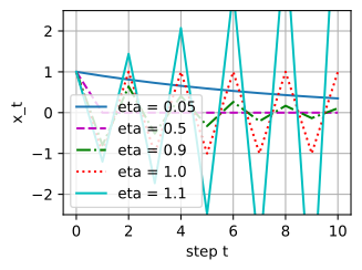
eta = 0.05 -> x_10 = +0.34868
eta = 0.50 -> x_10 = +0.00000
eta = 0.90 -> x_10 = +0.10737
eta = 1.00 -> x_10 = +1.00000
eta = 1.10 -> x_10 = +6.19174

Gradient descent on f(x) = x^2 (L = 2) from x_0 = 1, ten steps each.

Creep (\eta{=}0.05), one-shot (\tfrac12{=}1/L), zig-zag (0.9), bounce (1.0), diverge (1.1): the threshold \eta = 2/L is where the lemma’s guarantee expires.

Curvature & Taylor

the second derivative and the best polynomial

The second derivative is curvature

Curvature

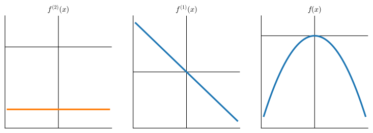
At a stationary point (f'=0) the sign of f'' decides the shape: up into a minimum, down into a maximum, flat is undecided. This is the second-derivative test.

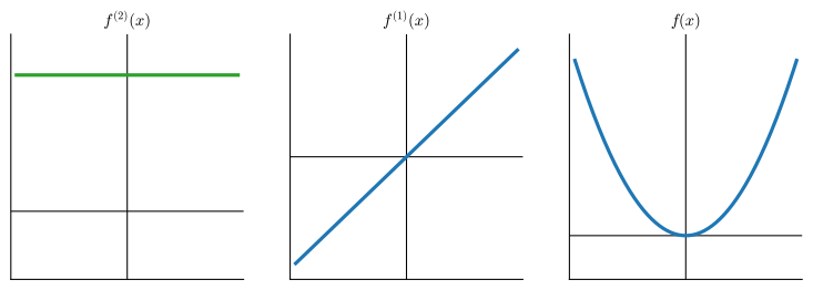
f'' > 0: slope rising, a bowl, local min.

f'' < 0: slope falling, a dome, local max.

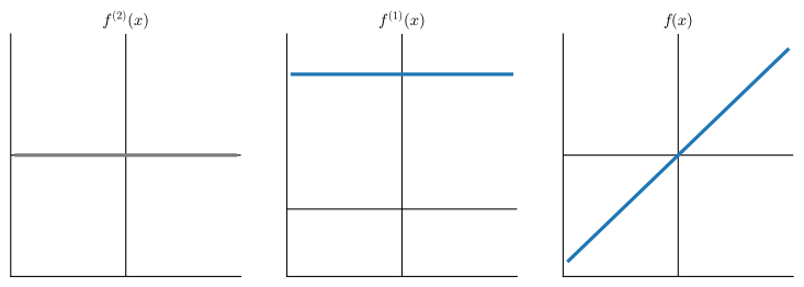
f'' = 0: slope constant, a line, inconclusive.

The Mean Value Theorem

Curvature

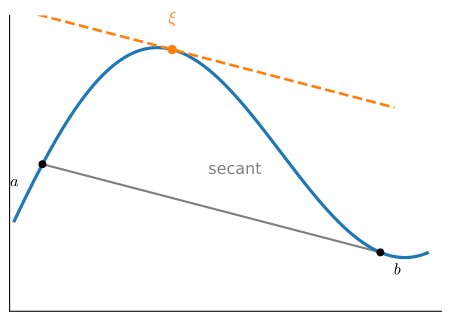
The bridge from the derivative at a point to the behavior of f on an interval: the average rate of change is hit exactly, somewhere inside.

f'(\xi) = \frac{f(b) - f(a)}{b - a}\quad\text{for some }\xi \in (a,b).

It is why a positive slope means f climbs, and what makes the Taylor remainder precise.

Some interior tangent runs parallel to the chord through the endpoints.

The best parabola → Newton’s method

Curvature

Matching value, slope, and curvature gives the best local parabola, which hugs the curve over a wider window than the tangent. It has a minimum of its own, so jump straight to it: Newton’s method x_{t+1} = x_t - f'(x_t)/f''(x_t).

This is gradient descent with \eta replaced by the curvature-adapted 1/f''(x_t): sharp curvature, caution; gentle, boldness.

The tangent matches value and slope; the best parabola also matches curvature.

Watch the digits double

Curvature

On f(x) = \tfrac14 x^4 - x, Newton’s method solves f'(x) = x^3 - 1 = 0 from x_0 = 2. Read the error column’s exponents: 10^{-2} \to 10^{-4} \to 10^{-8}.

# Newton's method on f(x) = x^4/4 - x: solve f'(x) = x^3 - 1 = 0, root x* = 1
x = 2.0
for t in range(6):
    print(f't = {t}: x = {x:.12f}, error = {abs(x - 1):.1e}')
    x = x - (x**3 - 1) / (3 * x**2)  # x - f'(x) / f''(x)

t = 0: x = 2.000000000000, error = 1.0e+00
t = 1: x = 1.416666666667, error = 4.2e-01
t = 2: x = 1.110534409842, error = 1.1e-01
t = 3: x = 1.010636768405, error = 1.1e-02
t = 4: x = 1.000111557304, error = 1.1e-04
t = 5: x = 1.000000012443, error = 1.2e-08

Each step roughly squares the previous error. Gradient descent shrinks the error by the same fixed factor every step, gaining a fixed number of digits; Newton doubles them.

Taylor series: the best degree-n polynomial

Curvature

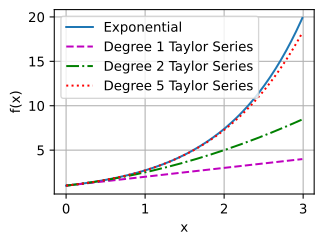
Matching the first n derivatives at x_0 gives the Taylor polynomial

P_n(x) = \sum_{i=0}^{n} \frac{f^{(i)}(x_0)}{i!}(x-x_0)^i.

For e^x at x_0 = 0, raising the degree visibly tightens the fit to the curve.

Each derivative adds a power of closeness

Curvature

The Lagrange remainder makes “the approximation improves near x_0” quantitative: the error shrinks like |x - x_0|^{n+1}, so halving the window should divide the worst error by 2^{n+1}:

n = 1: max error 2.1e-02 (h = 0.2) vs 5.2e-03 (h = 0.1), ratio = 4.1, prediction 2^2 = 4
n = 2: max error 1.4e-03 (h = 0.2) vs 1.7e-04 (h = 0.1), ratio = 8.2, prediction 2^3 = 8
n = 3: max error 6.9e-05 (h = 0.2) vs 4.3e-06 (h = 0.1), ratio = 16.3, prediction 2^4 = 16

The measured ratios land right on the predicted 4, 8, 16: each extra matched derivative adds a power of closeness, the wider-window effect measured.

Smooth is not analytic

Curvature

A warning before we lean on infinite series. The function f(x) = e^{-1/x^2} is smooth everywhere, yet every derivative at 0 vanishes.

Its Taylor series at 0 is identically zero: it converges on the whole line, but to the zero function, agreeing with f only at the origin. Convergence of the series is not convergence to f.

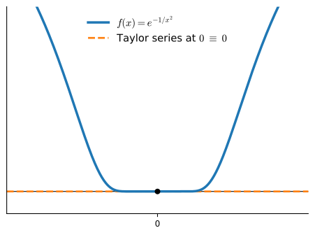
e^{-1/x^2} (solid) against its Taylor series at 0 (the zero line): smooth \ne analytic.

When the tangent fails

corners, subgradients, and stochastic training

Corners: no single tangent

Nonsmooth

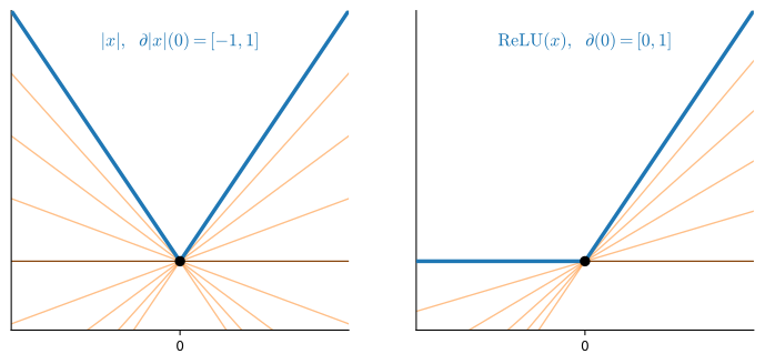
At each corner the one-sided slopes disagree; the subdifferential is the fan of all lines that stay below the graph.

At a corner (|x|, \mathrm{ReLU}) the one-sided slopes differ, so no single tangent exists. The subdifferential collects every valid slope:

\partial|x|(0) = [-1,1],\quad \partial\,\mathrm{ReLU}(0) = [0,1].

Optimality relaxes from f'(x)=0 to the inclusion 0 \in \partial f(x).

The split is in the difference quotient

Nonsmooth

The one-sided quotients of |x| at 0 are constants that never agree: +1 from the right, -1 from the left, so there is no limit to take. At the corner itself, autograd still answers:

# One-sided difference quotients of |x| at 0: constants, no limit needed
epsilon = 1e-4
print(f'right quotient: {(abs(epsilon) - abs(0)) / epsilon:+.1f}, '
      f'left quotient: {(abs(-epsilon) - abs(0)) / -epsilon:+.1f}')

# What autograd returns at the corner, where no derivative exists
for name, fn in [('d|x|/dx', jnp.abs), ("ReLU'", jax.nn.relu)]:
    print(f"{name} at 0: autograd returns {jax.grad(fn)(0.0):.1f}")

right quotient: +1.0, left quotient: -1.0
d|x|/dx at 0: autograd returns 1.0
ReLU' at 0: autograd returns 0.0

That gap is the corner: the two-sided derivative exists only when the one-sided slopes coincide. The 0 autograd returns is a convention, one fixed element of the set defined next.

The chain rule at a kink

Nonsmooth

At each kink, autograd returns one fixed element of the subdifferential (\mathrm{ReLU}'(0) = 0) and chains it through. But g(x) = \mathrm{ReLU}(x) - \mathrm{ReLU}(-x) is the identity, whose only correct slope at 0 is 1. Run it:

# g(x) = relu(x) - relu(-x) is the identity, so the true slope at 0 is 1
g = lambda x: jax.nn.relu(x) - jax.nn.relu(-x)
print(f"autograd: g'(0) = {jax.grad(g)(0.0):.1f}  (true slope: 1.0)")

autograd: g'(0) = 0.0  (true slope: 1.0)

Autograd reports slope 0 for the identity function: the chained convention 0 + 0 is not a subgradient of g at 0 at all, only an element of a conservative field.

Why SGD shrugs

Nonsmooth

The failure we just watched lives only at the kink, and the kinks form (heuristically) a measure-zero set.

Under a continuous sampling distribution, a fixed measure-zero set is hit with probability zero. Training iterates are data-dependent, however, and can land on kinks. Conservative-field convergence results cover many definable networks under their stated boundedness, step-size, and noise assumptions; they are not an unconditional guarantee for arbitrary nonsmooth training.

Recap

Wrap-up

Derivative = slope the curve flattens onto = limit of secants.
Small-change identity f(x+\epsilon)\approx f(x)+\epsilon f'(x) generates everything.
First-order term → gradient descent x \leftarrow x - \eta f'(x), safe for \eta < 2/L.

Second derivative = curvature; its sign is the min/max test.
Quadratic term → Newton’s method x_{t+1} = x_t - f'(x_t)/f''(x_t).
At corners use the subgradient (0 \in \partial f); kinks form a measure-zero set, so stochastic training is unaffected.