Differentiation in many variables the gradient · its geometry · the chain rule · the Hessian.
Derivatives with Many Parameters
Motivation
A deep network’s loss depends on millions to billions of weights, yet training rests on a single question: how does the loss change when we nudge the parameters?
The gradient\nabla_{\mathbf{w}} L is the answer, the derivative in many dimensions.
Its negative gives the direction of steepest descent, which underlies gradient-based optimization.
The chain rule, organized by the gradient, is backpropagation.
The Hessian tells a minimum from a saddle.
01
From partials to the gradient
one slope per coordinate, bundled into a vector
The gradient is the derivative
Gradients
Perturb every coordinate at once and discard the second-order cross terms, exactly as in one variable. The first-order term is a dot product:
This is f(x+\epsilon) \approx f(x) + \epsilon f'(x) with the scalar slope replaced by a vector and the product by a dot product. The gradient is the unique vector whose dot product with a step gives the first-order change in L.
Does the linear approximation hold?
Gradients
For f(x,y) = \log(e^x+e^y) at (0, \log 2), the gradient is [\tfrac13, \tfrac23]^\top. We compare the first-order prediction against the true value of a small step:
def f(x, y):return math.log(math.exp(x) + math.exp(y))def grad_f(x, y): s = math.exp(x) + math.exp(y)return [math.exp(x) / s, math.exp(y) / s]epsilon = [0.01, -0.03]x0, y0 =0, math.log(2)approx = f(x0, y0) +sum(e * g for e, g inzip(epsilon, grad_f(x0, y0)))true_value = f(x0 + epsilon[0], y0 + epsilon[1])print(f'approximation: {approx:.6f}, true value: {true_value:.6f}')
approximation: 1.081946, true value: 1.082124
They agree to about three decimals, and the gap of 1.8\times10^{-4} is itself the lesson: a first-order model discards terms of order \|\boldsymbol{\epsilon}\|^2 = 10^{-3} (the Hessian quadratic, coming up). Shrink the step tenfold and the gap shrinks a hundredfold.
Autograd reproduces the hand gradient:
autograd gradient: [0.33333334 0.6666667 ]
Directional Derivatives
Gradients
Read the approximation along a unit direction \mathbf{u} and the rate of change of L there (the directional derivative) is the gradient’s projection onto \mathbf{u}:
\frac{L(\mathbf{w} + h\,\mathbf{u}) - L(\mathbf{w})}{h} \;\xrightarrow{\,h\to 0\,}\; \mathbf{u}\cdot\nabla_{\mathbf{w}} L.
One vector \nabla_{\mathbf{w}} L encodes the slope in every direction simultaneously. The geometric results follow from this identity.
02
The geometry of gradients
steepest descent, level sets, tangent planes
Which way is steepest?
Geometry
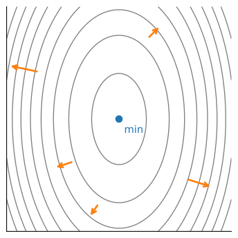
Along a unit direction \mathbf{v}, the change in L is \|\nabla L\|\cos\theta, so the direction enters only through \theta.
By Cauchy–Schwarz, -\|\nabla L\| \le \mathbf{v}\cdot\nabla L \le \|\nabla L\|: +\nabla L is steepest ascent, -\nabla Lsteepest descent.
Hence the gradient-descent step \mathbf{w} \leftarrow \mathbf{w} - \eta\,\nabla_{\mathbf{w}} L.
Linearization and Gradient Geometry
Geometry
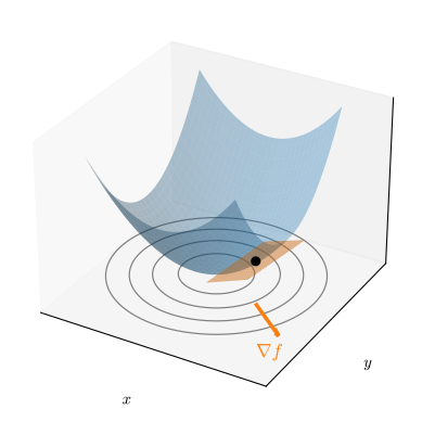
On the base plane, L does not change along a level set, so \nabla L is normal to the contours, longest where they bunch.
One dimension up, on the graph, the same equation is the tangent planez = f(\mathbf{x}_0) + \nabla f \cdot (\mathbf{x}-\mathbf{x}_0).
Drop the height coordinate and the surface normal becomes the gradient crossing the contours square on.
Where can a minimum be?
Geometry
If \nabla L(\mathbf{x}_0) \neq \mathbf{0}, stepping along -\nabla LlowersL, so \mathbf{x}_0 is no minimum. Contrapositively:
A minimum forces \nabla L(\mathbf{x}_0) = \mathbf{0}. Such points are critical points: necessary, not sufficient.
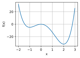
For f(x) = 3x^4-4x^3-12x^2, the critical points x=-1,0,2 have values -5, 0, -32; the plot confirms the minimum at x=2.
Optimizing under a constraint
Geometry
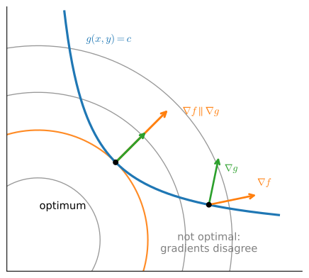
Minimize f subject to g(\mathbf{x}) = c. At the optimum no move along the constraint can lower f, so \nabla f is normal to \{g=c\}, and so is \nabla g. Two normals to one surface are parallel:
The level set of f is tangent to the constraint at the optimum: \lambda is the Lagrange multiplier, the seed of the KKT conditions and duality.
At the optimum the level set is tangent to the constraint and the gradients align; at the non-optimal point \nabla f keeps a component along the constraint, so sliding still improves f.
03
The chain rule and backprop
gradients are a sum over paths
Compositions are graphs
Chain rule
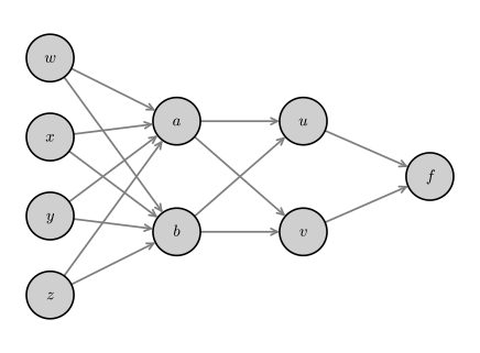
A network is a deep composition of simple functions. Drawn out, the dependencies form a graph: each node a value, each edge a direct functional dependence.
Substituting the full composite expression and differentiating it repeats the same subexpressions over and over. The chain rule organizes that waste away.
The rule is a sum over paths
Chain rule
Perturbing an input moves each intermediate by its partial. Reading off the first-order coefficient gives the whole rule:
Sum, over every directed path from input to output, the product of the edge derivatives along it.
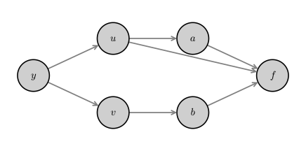
Here y reaches f by three paths, including a skip edge y\to u\to f, the same mechanism by which LSTM gates and residual connections shape gradient flow.
Forward-Mode Derivative Evaluation
Chain rule
Push an input forward through the graph and the single-step partials multiply out. One forward sweep returns only \partial f/\partial w, with no head start on the other inputs:
f at 1, 1, -2, 1 is 26896
df/dw at 1, 1, -2, 1 is 73472
Backward Evaluation of the Gradient
Chain rule
Walk the graph from the output backward, keeping \partial f in every numerator: compute \tfrac{\partial f}{\partial u}, \tfrac{\partial f}{\partial v} once, reuse them, and all four input derivatives fall out in a single sweep. This is backpropagation.
f at 1, 1, -2, 1 is 26896
df/dw at 1, 1, -2, 1 is 73472
df/dx at 1, 1, -2, 1 is 73472
df/dy at 1, 1, -2, 1 is -68224
df/dz at 1, 1, -2, 1 is -68224
Two sanity checks sit in the printout: \partial f/\partial w = \partial f/\partial x and \partial f/\partial y = \partial f/\partial z, as they must (f reaches its inputs only through w+x and y+z), yet the two pairs differ in size and sign, so the sweep genuinely tells the paths apart.
What autograd runs
Chain rule
The one-line autograd call runs exactly this backward pass. The four gradients match our by-hand sweep to the digit:
df/dw at [1.], [1.], [-2.], [1.] is [73472.]
df/dx at [1.], [1.], [-2.], [1.] is [73472.]
df/dy at [1.], [1.], [-2.], [1.] is [-68224.]
df/dz at [1.], [1.], [-2.], [1.] is [-68224.]
Why it is reverse-mode autodiff, a chain of vector–Jacobian products, is the matrix-calculus section.
04
Second-order: the Hessian
curvature tells a minimum from a saddle
The Hessian: curvature
Hessian
The gradient is first-order; the n^2 second partials determine curvature, collected into the Hessian\mathbf{H}_f.
Clairaut–Schwarz. If the mixed partials are continuous, order doesn’t matter: \partial^2 f/\partial x_i\partial x_j = \partial^2 f/\partial x_j\partial x_i, so \mathbf{H}_f = \mathbf{H}_f^\top.
Because \mathbf{H} is symmetric, the spectral theorem applies and supports the second-derivative test.
The best-fitting quadratic
Hessian
Just as the gradient gives the best linear fit, the Hessian gives the best quadratic fit, the second-order Taylor approximation:
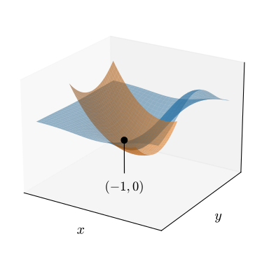
Near \mathbf{x}_0 the surface and the quadratic are nearly indistinguishable, separating only farther out.
Checking the quadratic
Hessian
Stepping from the base point (-1, 0), the gap between f and its Taylor quadratic q stays tiny nearby and grows with distance:
step 0.00: f = -0.367879, quadratic = -0.367879, gap = 0.000000
step 0.05: f = -0.384315, quadratic = -0.384434, gap = 0.000119
step 0.10: f = -0.396388, quadratic = -0.397310, gap = 0.000921
step 0.30: f = -0.391929, quadratic = -0.412025, gap = 0.020096
The gap is third order (double the step, eight times the gap), which is what the local quadratic guarantee predicts. Newton’s method minimizes this model when it is positive definite and safeguards the step otherwise.
The second-derivative test
Hessian
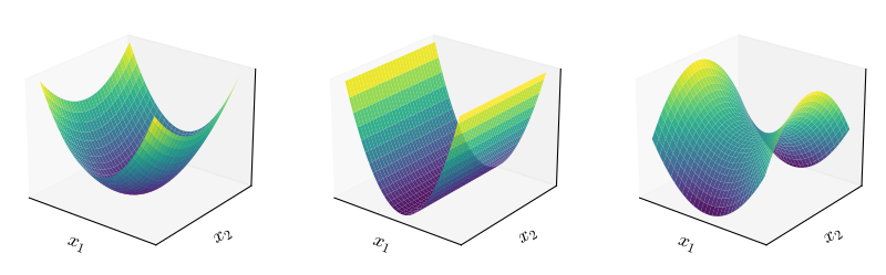
At a critical point the picture is purely quadratic; the curvature \mathbf{v}^\top\mathbf{H}\mathbf{v} along \mathbf{v} gives the second-order test through the definiteness of \mathbf{H}, read off its eigenvalues:
\mathbf{H}\succ0 → minimum (bowl). \mathbf{H}\prec0 → maximum. Mixed signs → saddle. A zero eigenvalue → second order is silent.
The test, run as a program
Hessian
The surface f(x,y) = x\,e^{-x^2-y^2} has exactly two critical points, (\pm 1/\sqrt{2},\, 0). Assemble each Hessian from symmetric second differences, read off the 2\times2 eigenvalues, and classify:
at (-0.7071, 0): eigenvalues +0.858, +1.716 -> minimum
at (+0.7071, 0): eigenvalues -1.716, -0.858 -> maximum
Differentiate twice, extract eigenvalues, read the signs: all positive is a minimum, all negative a maximum, and a saddle shows one of each.
Saddle Points in High Dimensions
Hessian
A minimum needs alln eigenvalues positive at once. If their signs behaved like coin flips, that is probability 2^{-n}, vanishing in high dimension.
So the critical points met while training deep nets are overwhelmingly saddles, not the bad local minima once feared, one reason gradient methods do so well in practice.
The gradient represents Euclidean linear change
Wrap-up
The gradient is the derivative in many dimensions: \boldsymbol{\epsilon}\cdot\nabla L is the first-order change, and its projection gives the slope in any direction.
-\nabla L is steepest descent, and \nabla L \perp the level sets: the geometry of gradient descent.
The chain rule sums products of edge derivatives over paths; run backward it reuses everything: that is backpropagation.
The symmetric Hessian gives the quadratic fit; its eigenvalues separate minimum, maximum, and saddle.
Every optimizer in this book (GD, momentum, Adam, Newton) reads the local Taylor expansion of the loss and moves against the gradient.