Row i collects the partials of output i; column j says how every output reacts to nudging input j.
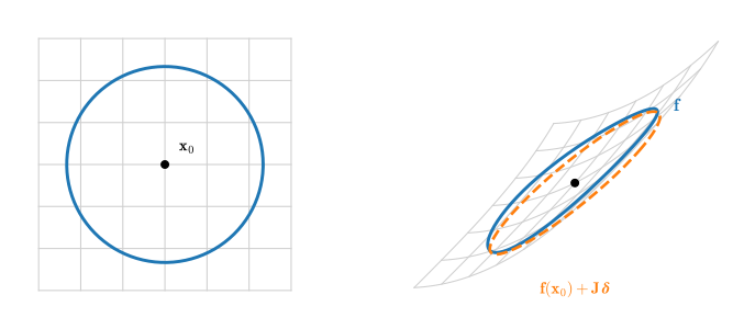
A small circle of inputs maps to an approximate ellipse, its image under \mathbf J. The leftover bend is the o(\|\boldsymbol\delta\|) remainder.
Jacobians, Gradients, and Hessians
The Jacobian
The Jacobian unifies the derivative objects introduced so far:
Scalar map (m=1): \mathbf J is one row, the gradient \partial f/\partial\mathbf x.
Vector map: the full m\times n matrix of partials.
Hessian: the Jacobian of the gradient field, \mathbf H=\mathbf J_{\nabla f}.
One construction recovers the slope, the gradient, and the matrix of second derivatives.
The numerical signature of a derivative
The Jacobian
The linear model must beat its own error: halve \boldsymbol\delta and the error should fall fourfold. Check \mathbf f(x,y)=(x^2y,\ \sin(x+y)) against a finite difference, prediction vs truth:
The error relative to \|\boldsymbol\delta\| is tiny, and shrinking \boldsymbol\delta tenfold shrinks it a hundredfold: the o(\|\boldsymbol\delta\|) fingerprint.
02
The chain rule is Jacobian composition
multiplication of matrices, in any order
Composition multiplies Jacobians
Chain rule
The multivariate chain rule (a sum over paths) is, in matrix form, just a product of Jacobians:
A depth-L network is a composition \mathbf f_L\circ\cdots\circ\mathbf f_1, so its end-to-end derivative is one long matrix product, one local Jacobian per layer.
Two shapes dominate the product
Chain rule
Real networks alternate just two kinds of factor:
Dense\mathbf x\mapsto\mathbf W\mathbf x
Its own best linear map, so \mathbf J=\mathbf W.
Elementwise\boldsymbol\varphi
Couples no coordinates, so \mathbf J=\operatorname{diag}(\varphi').
So \mathbf J=\operatorname{diag}(\boldsymbol\varphi_L')\,\mathbf W_L\cdots\operatorname{diag}(\boldsymbol\varphi_1')\,\mathbf W_1: weights interleaved with cheap diagonal masks. For ReLU that mask is just zeros and ones, which is why a backward pass through an activation costs O(n).
Associativity: two brackets, two modes
Chain rule
Matrix multiplication is associative, so the chain \mathbf J_L\cdots\mathbf J_1 may be bracketed in any order:
For a dense derivative product, the two modes are alternative parenthesizations; graph reuse, sparsity, batching, and memory can change the practical cost.
03
Identities, derived not tabulated
differentiate one component, reassemble
Four identities, one method
Identities
Differentiate one component, reassemble, then sanity-check the 1\times1scalar collapse:
\nabla_{\mathbf x}\,\mathbf a^\top\mathbf x = \mathbf a
\nabla_{\mathbf x}\,\mathbf x^\top\mathbf A\mathbf x = (\mathbf A+\mathbf A^\top)\mathbf x
softmax + cross-entropy, w.r.t. the logits =\mathbf p-\mathbf y
No table needed: the least-squares gradient is the rank-one outer product a linear layer returns in backprop.
Derive, then verify: autograd audits the first two at a random point:
grad a^T x   equals a        : True
grad x^T A x equals (A+A^T)x : True
The cancellation that fuses softmax with cross-entropy
Identities
The softmax Jacobian \operatorname{diag}(\mathbf p)-\mathbf p\mathbf p^\top, composed with cross-entropy, collapses to \mathbf p-\mathbf y whatever the Jacobian; the fused softmax–cross-entropy primitive also avoids \log of an underflowed probability via log-sum-exp. Verify against autograd:
The \varepsilon-coefficient ad+bcis the product rule. So running a program on x+1\cdot\varepsilon yields
f(x+\varepsilon)=f(x)+f'(x)\,\varepsilon.
The same pass computes the derivative: seed the input’s \varepsilon-part with 1 and read the output’s \varepsilon-part.
Dual Numbers in Python
Forward mode
A handful of overloaded operators is forward-mode AD: the \varepsilon-part returns f'(x)=2x\cos(x^2)+e^x in one pass, no formula for f' written. Differentiate f(x)=\sin(x^2)+e^x at x=1.3:
def f(x):return (x * x).sin() + x.exp() # sin(x^2) + e^x, in dual algebrax0 =1.3out = f(Dual(x0, 1.0)) # seed the derivative with 1exact =2* x0 * np.cos(x0**2) + np.exp(x0) # f'(x) by handprint('dual result :', out)print('value f(x) :', np.sin(x0**2) + np.exp(x0))print("derivative : dual %.6f vs exact %.6f"% (out.b, exact))
dual result : 4.662200 + 3.360101 eps
value f(x)  : 4.662200318713363
derivative  : dual 3.360101  vs  exact 3.360101
One pass per input: cheap when tall
Forward mode
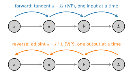
With a vector tangent, one forward pass carries a Jacobian–vector product\mathbf J\mathbf v, a linear combination of columns, never forming \mathbf J. Seeding \mathbf e_j reads off literal columnj.
Forward mode costs one pass per input. It is efficient for tall Jacobians (m\gg n) but inefficient for a scalar loss over millions of inputs.
05
Reverse mode, the tape, and backprop
record forward, replay backward
Why reverse mode is the right cost model
Reverse mode
Reverse mode multiplies left-to-right, carrying a vector–Jacobian product\mathbf u^\top\mathbf J, one pass per output.
A scalar loss is a single-row Jacobian (m=1), so one backward sweep yields the entire gradient.
Gradient of a scalar in one reverse sweep at a small constant multiple of the primal cost: the cheap-gradient principle (Baur–Strassen).
One row or one column per pass
Reverse mode
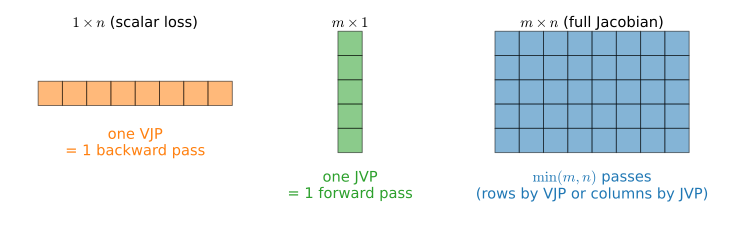
The cost rule, drawn as shapes. A pass buys one row (reverse, a VJP) or one column (forward, a JVP); the cheap mode is the one whose unit matches your Jacobian’s short side.
A scalar loss is one row: one VJP, one backward pass. The full m\times n matrix costs \min(m,n) passes either way, which is why it is never formed.
The tape: a diamond, not a chain
Reverse mode
Record each op as a node with a backward closure; replay in reverse topological order, seeding the output adjoint with 1.
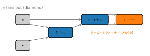
For r=uv+u, y=r^2, the value r feeds both arguments of y, so its adjoint arrives twice.
A node’s adjoint is the sum over its outgoing edges, the chain rule’s “sum over paths”, which is why the tape accumulates with +=, not =.
Thirty lines reproduce the backward pass
Reverse mode
One forward pass records the tape; one backward pass yields both partials, matching the framework’s own autograd. Real engines use tensor nodes, VJP rules, and a larger primitive set, but follow the same procedure:
u, v = Var(2.0), Var(-3.0)r = u * v + u # shared intermediatey = r * r # r feeds both argumentsbackprop(y)ut = torch.tensor(2.0, requires_grad=True)vt = torch.tensor(-3.0, requires_grad=True)rt = ut * vt + ut(rt * rt).backward() # framework autogradprint('our tape : dy/du = %.4f dy/dv = %.4f'% (u.grad, v.grad))print('torch : dy/du = %.4f dy/dv = %.4f'% (ut.grad, vt.grad))
The two engines make the pass-count difference measurable. Take a scalar function of n = 200 inputs: forward mode assembles the gradient one input direction per pass; the tape runs one backward sweep.
forward mode : 200 passes (one per input)
reverse mode : 1 backward sweep for all 200 partials
max |forward - reverse| over the gradient: 0.0e+00
Identical gradients, a factor-n gap in pass counts; per-pass costs match to a small constant, so the work ratio is \Theta(n). Replace 200 by the 10^8 parameters of a modern network: that factor is why no framework trains in forward mode.
Products Without Explicit Jacobians
Reverse mode
A dense m\times n Jacobian costs \min(m,n) passes and \Theta(mn) storage; a JVP or VJP costs one pass and stores only a vector.
Most derivative calculations require only the action of a Jacobian. Autograd exposes JVPs and VJPs so these actions can be composed without assembling the matrix.
One order up, the Hessian–vector product\mathbf H\mathbf v is the directional derivative of the gradient map: curvature in a direction without ever forming \mathbf H.
Hessian–Vector Products
Reverse mode
Differentiate the gradient once, in one direction. For L(\mathbf x) = \tfrac12\mathbf x^\top\mathbf A\mathbf x the Hessian is \mathbf A itself, so the expected product is known in advance, and no 2\times2 matrix of second derivatives is ever assembled:
# Hv for L(x) = x^T A x / 2, where H = A exactlyA = jnp.array([[3.0, 1.0], [1.0, 2.0]])L =lambda x: 0.5* x @ A @ xx, v = jnp.array([1.0, -2.0]), jnp.array([1.0, 0.5])_, Hv = jax.jvp(jax.grad(L), (x,), (v,)) # forward over reverseprint('forward-over-reverse Hv:', Hv)print('A v :', A @ v)
forward-over-reverse Hv: [3.5 2. ]
A v                    : [3.5 2. ]
Cost: a small constant multiple of one gradient, rather than n gradients. The absolute cost still follows the primal computation. This is what makes Newton and conjugate-gradient methods, and curvature diagnostics, tractable at scale.
Differentiating through an equation
Reverse mode
Some outputs are defined implicitly: \mathbf x^\star(\boldsymbol\theta) solves \mathbf g(\mathbf x^\star, \boldsymbol\theta) = \mathbf 0 (a fixed point, an equilibrium, an inner argmin). No need to tape the solver.
Implicit function theorem. Differentiating the identity \mathbf g(\mathbf x^\star(\boldsymbol\theta), \boldsymbol\theta) \equiv \mathbf 0 gives \;\frac{\partial\mathbf x^\star}{\partial\boldsymbol\theta} = -\bigl(\frac{\partial\mathbf g}{\partial\mathbf x}\bigr)^{-1}\frac{\partial\mathbf g}{\partial\boldsymbol\theta}, both Jacobians at the solution only.
One linear solve per gradient, however many iterations the solver ran. Checked on a 2\times2 Newton solve, against a finite difference of the solver’s output:
The derivative depends on the defining equation rather than the solver trajectory. This principle underlies the adjoint method, deep equilibrium models, and bilevel optimization.
Tape Memory and Checkpointing
Reverse mode
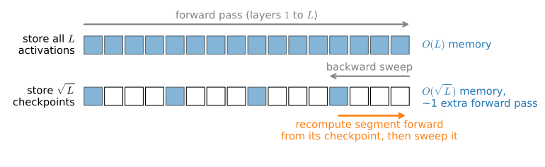
Reverse mode must keep every forward intermediate alive until the backward sweep consumes it: O(L) activation memory, often the binding constraint on batch size and depth.
Checkpointing stores only every \sqrt{L}-th activation and recomputes each segment when the sweep reaches it: O(\sqrt{L}) memory for roughly one extra forward pass.
JVPs and VJPs compute derivative actions
Wrap-up
The Jacobian is the best local linear map; the gradient (m=1) and the Hessian are special cases.
The chain rule is Jacobian composition; a deep net is one long matrix product.
Its associativity is what yields the two autodiff modes.
Forward mode (dual numbers, JVP): one column per pass, cheap when tall.
Reverse mode (the tape, VJP): one row per pass, cheap when wide. A loss is maximally wide, so backprop is reverse-mode AD, paid for in stored activations (checkpointing buys them back).
Compose, never assemble:\mathbf H\mathbf v by differentiating the gradient; implicit outputs by one linear solve.
JVPs and VJPs provide the derivative actions used by gradients, Hessian–vector products, and implicit differentiation without assembling full Jacobians.