Integral Calculus

Dive into Deep Learning · §25.4

Accumulation over intervals and regions
Riemann sums · the fundamental theorem · change of variables · probability.

Why integration

Motivation

Differentiation describes the local change in f under a perturbation of x. Integration accumulates a quantity over an interval or region, and the fundamental theorem relates the two operations.

An area under a curve, a volume under a surface.
Every continuous probability is an integral, \int p = 1.
Every expectation is an integral average, \int x\,p(x)\,dx.
The change-of-variables rule computes the Gaussian normalizer.

The integral and the theorem

a limit of sums, and how to compute it

The definite integral as a limit

The integral

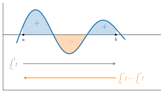
Choose a tagged partition P of [a,b]. If every choice of tags converges to the same value as the largest subinterval shrinks, then f is Riemann integrable and

\int_a^b f(x)\,dx = \lim_{\|P\|\to0}\sum_i f(\xi_i)(x_i-x_{i-1}).

Equal-width rectangles are one special sequence; values below the axis contribute negatively.

Convergence of Riemann Sums

The integral

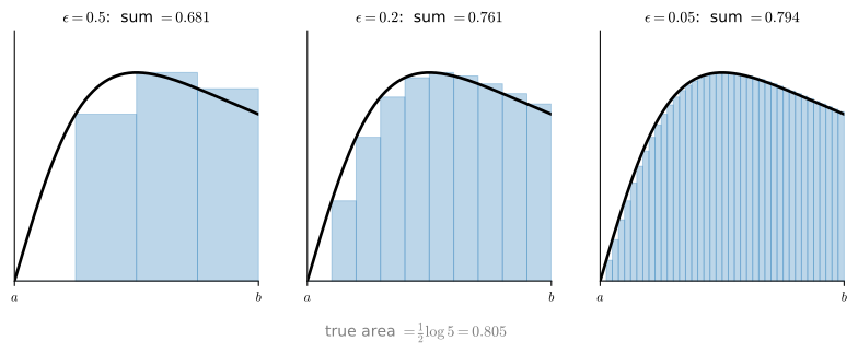
The definition converges, but slowly. Refine the partition for \int_0^2 \tfrac{x}{1+x^2}\,dx = \tfrac12\log 5 and the left-rule error shrinks in step with \epsilon:

eps=0.5    sum=0.680769  error=0.123950
eps=0.1    sum=0.783785  error=0.020934
eps=0.05   sum=0.794486  error=0.010233
eps=0.01   sum=0.802710  error=0.002009
eps=0.001  sum=0.804519  error=0.000200
truth = (1/2) log 5 = 0.804719

First-order convergence: cut \epsilon by ten, cut the error by ten. The procedure is slow and produces no closed form.

The fundamental theorem of calculus

The integral

Let the upper limit vary. The area-so-far function F(x)=\int_a^x f accumulates signed area out to x. Nudge x by \epsilon and only one thin sliver of new area appears, of height f(x), so

\frac{dF}{dx}(x) = f(x).

The rate at which area grows is the current height. Finding areas becomes the search for an antiderivative.

Integration is differentiation reversed

The integral

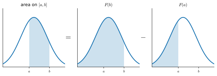
If G'=f then every definite integral is a difference of two values:

\int_a^b f(x)\,dx = G(b) - G(a).

The limit of sums becomes an antiderivative evaluation. We check it numerically: build F as a cumulative Riemann sum, finite-difference it, and compare against f itself.

max |dF/dx - f|      : 5.551115123125783e-14
Riemann F(2) vs G(2)-G(0): 0.8045188628837103 0.8047189562170501

The error is float32 roundoff, not discretization: differencing the cumulative sum telescopes back to the term it just added.

Improper integrals

The integral

Densities live on unbounded domains, so we integrate to infinity as a limit, \int_a^\infty f = \lim_{b\to\infty}\int_a^b f. The power law is the test case:

\int_1^\infty x^{-p}\,dx = \begin{cases}\dfrac{1}{p-1}, & p>1\ \text{(converges)},\\[1ex]\infty, & p\le 1\ \text{(diverges)}.\end{cases}

The threshold p=1 decides whether a heavy-tailed density has a finite normalizer or mean at all.

Truncation and Discretization Error

The integral

Evaluate the convergent improper integral \int_0^\infty e^{-x}\,dx=1 using two approximations: the exact partials 1-e^{-b} and a left-Riemann sum of each:

b=1.0   left-Riemann sum=0.632437  exact 1-e^-b=0.632121
b=2.0   left-Riemann sum=0.865097  exact 1-e^-b=0.864665
b=5.0   left-Riemann sum=0.993759  exact 1-e^-b=0.993262
b=10.0  left-Riemann sum=1.000455  exact 1-e^-b=0.999955
b=20.0  left-Riemann sum=1.000500  exact 1-e^-b=1.000000

The partials approach 1 as b grows (truncation error e^{-b}); the left rule settles near 1.0005, not 1 (discretization error \approx\tfrac{\epsilon}{2}). The error sources are independent; reducing one does not reduce the other.

Integration by parts

The integral

The product rule, run backwards through the theorem:

\int_a^b u\,v'\,dx = \bigl[\,u\,v\,\bigr]_a^b - \int_a^b u'\,v\,dx.

Move the derivative onto the factor that can absorb it. With u=x, v'=e^{-x},

\int_0^\infty x\,e^{-x}\,dx = \bigl[\,-x\,e^{-x}\,\bigr]_0^\infty + \int_0^\infty e^{-x}\,dx = 1,

the mean of the exponential, and the move behind score matching’s Hyvärinen identity.

Area comes with a sign

The integral

Two independent sign rules govern \int_a^b f:

where f<0, area counts negative: \int_0^1 (-1)\,dx = -1
reversing the limits negates: \int_b^a f = -\int_a^b f

Each flip contributes one minus sign, and two cancel: \int_0^{-1}(-1)\,dx = +1.

The same sign convention the determinant used for transformed areas, and exactly what makes change of variables come out right.

Lobes above the axis count positive, the lobe below counts negative; reversing the limits traverses the same area backwards and negates the total.

Change of variables

the chain rule, run backwards

Substitution in one dimension

Change of variables

Reparametrize through y=u(x). A sliver of width \epsilon at x maps to one of width \epsilon\,u'(x), so matching areas forces the local stretch factor:

\int_{u(a)}^{u(b)} f(y)\,dy = \int_a^b f(u(x))\,\frac{du}{dx}\,dx.

A suitable u reduces the original integral to a known form.

Multiple integrals

double integrals, Fubini, the Jacobian, and the Gaussian

Multiple integrals: a volume under a surface

Double integrals

For f(x,y) on a box, \int_U f\,d\mathbf{x} is the volume between the surface and the base plane. The Riemann approximation tiles the base with \epsilon\times\epsilon squares and sums the corresponding box volumes.

Our running example is the bell e^{-x^2-y^2} over [-2,2]^2.

The box volume, numerically

Double integrals

Total the boxes on a fine grid over [-2,2]^2. The exact value involves the error function \operatorname{erf}, the Gaussian’s antiderivative, which has no elementary formula but ships as a library routine:

Riemann volume over the box [-2, 2]^2 : 3.11227
exact volume  pi * erf(2)^2           : 3.11227

Over the whole plane the volume becomes exactly \pi, computed below.

Fubini: sum in any order

Fubini

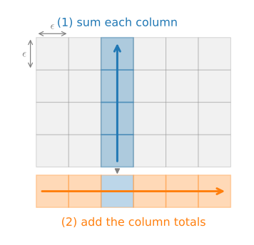
A grid sum totals in any order. Summing columns-first and passing to the limit splits the double integral into iterated single ones:

\int_U f\,dx\,dy = \int\!\!\left(\int f\,dx\right)dy = \int\!\!\left(\int f\,dy\right)dx.

(Needs f absolutely integrable, \int_U |f| < \infty; the rule in machine learning.)

Change of variables in many dimensions

Change of variables

For a C^1-diffeomorphism \boldsymbol{\phi}, the scalar stretch \tfrac{du}{dx} becomes the Jacobian determinant:

\int_{\boldsymbol{\phi}(U)}\! f\,d\mathbf{x} = \int_{U}\! f(\boldsymbol{\phi}(\mathbf{x}))\,\bigl|\det D\boldsymbol{\phi}\bigr|\,d\mathbf{x}.

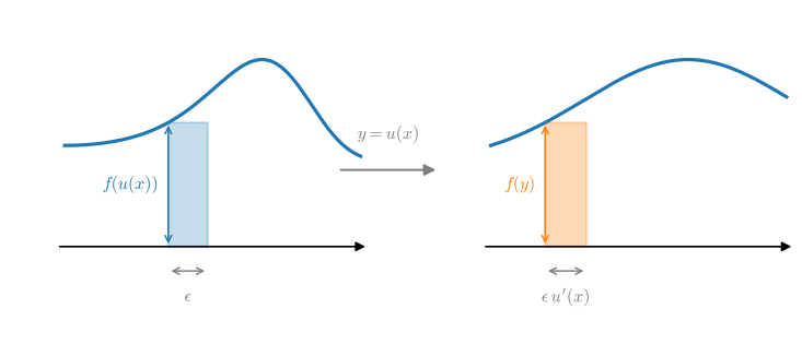
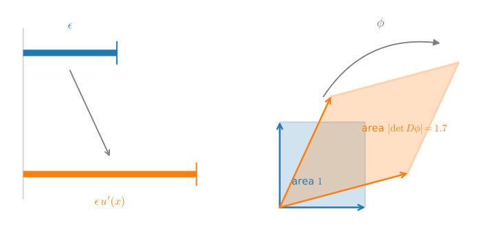
The determinant is exactly the factor by which a linear map scales volume, so a tiny cube of volume d\mathbf{x} becomes a parallelepiped of volume |\det D\boldsymbol{\phi}|\,d\mathbf{x}.

Read for densities instead of areas, this same factor (as -\log|\det D\boldsymbol{\phi}|) underlies normalizing flows.

The Gaussian integral

The one-dimensional \int_{-\infty}^\infty e^{-x^2}\,dx has no elementary antiderivative. Go up a dimension: square it, merge the copies by Fubini, then switch to polar coordinates,

\left(\int e^{-x^2}\,dx\right)^{\!2} = \iint e^{-x^2-y^2}\,dx\,dy = \int_0^\infty\!\!\int_0^{2\pi}\! r\,e^{-r^2}\,d\theta\,dr = \pi.

The polar map contributes Jacobian |\det D\boldsymbol{\phi}|=r, the factor that makes the integrand elementary. So \int e^{-x^2}\,dx=\sqrt\pi:

grid integral of e^(-x^2-y^2): 3.141593
exact value pi               : 3.141593

Integration meets probability

densities, expectations, and Monte Carlo

Densities and expectations

Probability

This is why a deep-learning reader needs integration. A continuous density is a non-negative function that is normalized; an expectation is an integral average:

\int_{\mathcal X} p = 1, \qquad \mathbb{E}[g(X)] = \int_{\mathcal X} g(x)\,p(x)\,dx.

The Gaussian integral supplies the normalizer: p(x)=\tfrac{1}{\sqrt\pi}e^{-x^2} integrates to 1, and symmetry sends its mean to 0.

total mass  integral p dx : 1.0
mean        integral x p dx: 0.0

Monte Carlo in High Dimensions

Probability

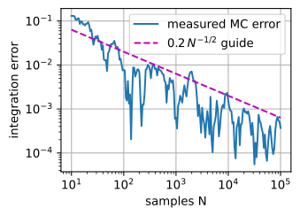
With no closed form, Monte Carlo estimates an expectation by sampling, \mathbb{E}[g(X)] \approx \tfrac1n\sum_i g(x_i), at rate 1/\sqrt n in every dimension (the constant, the standard deviation of g(X), may grow with d; the exponent never does).

A grid to resolution \epsilon in d dimensions costs N=\epsilon^{-d} points and decays only as N^{-2/d}: the exponent is divided by d. In moderate or high dimensions, sampling is generally more practical than a uniform grid.

n=10      Monte Carlo=0.87741  error=1.3e-01
n=100     Monte Carlo=0.75454  error=7.7e-03
n=1000    Monte Carlo=0.74619  error=6.3e-04
n=10000   Monte Carlo=0.74833  error=1.5e-03
n=100000  Monte Carlo=0.74719  error=3.7e-04
midpoint quadrature  =0.74682

Differentiating under the integral

Probability

Training through an expectation means swapping \nabla_{\boldsymbol\theta} and \int; the plain swap is what shows the score \nabla_{\boldsymbol\theta}\log p_{\boldsymbol\theta} has mean zero, the identity at the heart of policy gradients. When the limits move too, the Leibniz rule adds the boundary terms:

\frac{d}{d\theta}\!\int_{a(\theta)}^{b(\theta)}\! f(x,\theta)\,dx = \int_{a(\theta)}^{b(\theta)}\!\frac{\partial f}{\partial\theta}\,dx + f(b(\theta),\theta)\,b'(\theta) - f(a(\theta),\theta)\,a'(\theta).

Each moving endpoint sweeps area in or out at the rate it moves, weighted by the integrand’s value there.

For a density supported on [0,\theta], omitting the boundary term produces an incorrect gradient.

Integration accumulates signed contributions

Wrap-up

Integral = signed area or volume, a limit of Riemann sums.
Fundamental theorem: F'=f, so integration is the inverse of differentiation, \int_a^b f = G(b)-G(a).
By parts: \int u\,v' = [\,uv\,] - \int u'\,v moves a derivative onto the factor that can absorb it.

Change of variables scales by du/dx in 1-D, the Jacobian |\det D\boldsymbol{\phi}| in n-D, the volume-scaling factor of the map.
Fubini evaluates a multiple integral as iterated single ones.
Probability: a density is \int p = 1; an expectation is an integral, estimated by Monte Carlo when it has no closed form.