Weight Decay

Dive into Deep Learning · §2.7

Taming overfitting by shrinking the weights
the \ell_2 penalty · the geometry · the spectral why · the Bayesian reading.

When more data is not an option

Motivation

• Overfitting fades with more data, but data is often costly or fixed.
• Dropping features is too blunt: with k inputs there are \binom{k-1+d}{k-1} degree-d monomials.
• Instead, restrict the values the weights may take.

Among all f, the constant f=0 is the simplest. Measure complexity by how far the weights sit from zero.

\|\mathbf{w}\|_2^2 = \sum_i w_i^2

A single number that grows as the weights stretch away from the origin.

Add the size of the weights to the loss

The idea

Penalize a large weight vector by adding its squared norm to the objective, scaled by a knob \lambda \ge 0:

L(\mathbf{w}, b) \;+\; \frac{\lambda}{2}\,\|\mathbf{w}\|_2^2.

• \lambda = 0 recovers the plain loss; larger \lambda pulls \mathbf{w} harder toward zero.
• The \tfrac{1}{2} is cosmetic: it cancels the 2 from differentiating the square.

\ell_2-regularized linear regression is the classic ridge regression; the \ell_1 version is lasso.

Ridge shrinks, lasso selects

The geometry

A budget \|\mathbf{w}\| \le t turns the penalty into a constraint: the answer is where a loss contour first touches the constraint region.

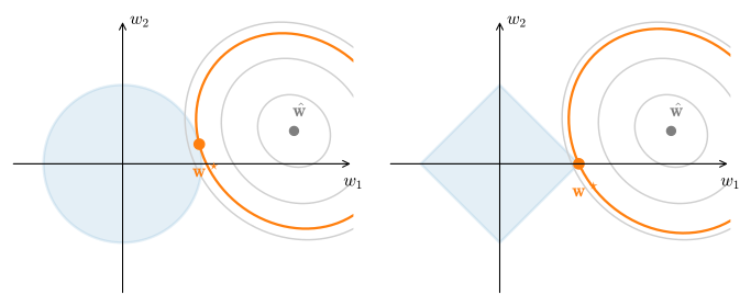
Loss contours centred on the unconstrained optimum \hat{\mathbf{w}} grow until they meet the constraint at \mathbf{w}^\star. Left (\ell_2 ball): contact is tangential, so both coordinates shrink. Right (\ell_1 diamond): contact is at a corner, forcing w_2 to exactly zero.

A round ball touches off-axis (everything shrinks); a pointed diamond touches at a corner (sparsity). This is why lasso does feature selection and ridge does not.

Why it is called weight decay

The update

The penalty adds \lambda\mathbf{w} to the gradient, so each SGD step gains a shrink factor:

\mathbf{w} \leftarrow (1 - \eta\lambda)\,\mathbf{w} \;-\; \frac{\eta}{|\mathcal{B}|}\!\sum_{i \in \mathcal{B}} \mathbf{x}^{(i)}\bigl(\mathbf{w}^\top\mathbf{x}^{(i)} + b - y^{(i)}\bigr).

Before fitting the data at all, every weight is decayed toward zero by the factor 1 - \eta\lambda.

\lambda is a continuous complexity dial: unlike deleting features, it never forces a hard choice.

Usually the bias is left undecayed.

01

From Scratch

a problem built to overfit, then regularized

A regression rigged to overfit

From Scratch

A tiny linear signal in 200 inputs plus faint noise, y = 0.05 + \sum_i 0.01\,x_i + \epsilon:

class Data(d2l.DataModule):
    def __init__(self, num_train, num_val, num_inputs, batch_size):
        self.save_hyperparameters()                
        n = num_train + num_val 
        key_X, key_noise = jax.random.split(jax.random.key(0))
        self.X = jax.random.normal(key_X, (n, num_inputs))
        noise = jax.random.normal(key_noise, (n, 1)) * 0.01
        w, b = d2l.ones((num_inputs, 1)) * 0.01, 0.05
        self.y = d2l.matmul(self.X, w) + b + noise

    def get_dataloader(self, train):
        i = slice(0, self.num_train) if train else slice(self.num_train, None)
        return self.get_tensorloader([self.X, self.y], train, i)

20 examples for 200 parameters: 10× more knobs than data. Overfitting is guaranteed by design, so its remedy is unmistakable.

The penalty, then the model

From Scratch

The penalty is a single line:

def l2_penalty(w):
    return d2l.reduce_sum(w**2) / 2

Subclass the scratch regressor and fold it into the loss:

class WeightDecayScratch(d2l.LinearRegressionScratch):
    def __init__(self, num_inputs, lambd, lr, sigma=0.01, rngs=None):
        super().__init__(num_inputs, lr, sigma, rngs=rngs)
        self.save_hyperparameters(ignore=['rngs'])

    def loss(self, y_hat, y):
        return (super().loss(y_hat, y) +
                self.lambd * l2_penalty(self.w))

Nothing else changes: same linear model, same squared loss. The penalty rides along, scaled by lambd.

\lambda = 0: the overfit, on display

From Scratch · the overfit

train_scratch(0)

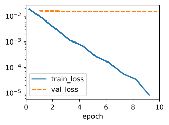
L2 norm of w: 0.010900449939072132

Training loss plunges; validation loss never follows, and the printed \|\mathbf{w}\|^2 shows the price of that perfect memory. A textbook overfit.

\lambda = 3: the rescue

From Scratch · the rescue

train_scratch(3)

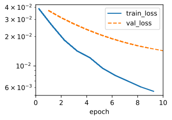
L2 norm of w: 0.0007385745993815362

Training loss is higher (we forbade memorization) but validation loss finally falls, with \|\mathbf{w}\|^2 an order of magnitude smaller.

Why shrinkage helps: damp the directions the data cannot see

From Scratch · the why

Ridge keeps a closed form, and the SVD \mathbf{X} = \mathbf{U}\mathbf{D}\mathbf{V}^\top shows exactly what shrinks: the response along the j-th principal direction is damped by

\frac{d_j^2}{d_j^2 + \tilde{\lambda}} \qquad\Rightarrow\qquad \textrm{df}(\tilde{\lambda}) = \sum_j \frac{d_j^2}{d_j^2 + \tilde{\lambda}}.

Strong directions (d_j large) pass through nearly untouched; the weakly constrained ones are suppressed hardest.

Twenty examples pin down at most 20 of 200 directions (\textrm{df}(0) = 20); \lambda = 3 prices the model at \textrm{df} \approx 15 effective parameters.

02

The Built-In Way

where the framework keeps the decay

Decay as a gradient transform

Concise · JAX

Optax has no weight_decay in sgd, so we chain transforms and mask the decay to the kernel. add_decayed_weights injects \lambda\mathbf{w} into the gradient; the mask spares the bias.

class WeightDecay(d2l.LinearRegression):
    def __init__(self, wd, lr, num_inputs=200, rngs=None):
        super().__init__(num_inputs, lr, rngs=rngs)
        self.save_hyperparameters(ignore=['rngs'])

    def configure_optimizers(self):
        # Weight Decay is not available directly within optax.sgd, but
        # optax allows chaining several transformations together. We
        # mask the decay so it applies to the kernel only (not bias),
        # matching the per-parameter-group convention in PyTorch / MXNet.
        def kernel_mask(params):
            return jax.tree_util.tree_map_with_path(
                lambda path, _: getattr(path[-1], 'name', None) == 'kernel',
                params)
        return optax.chain(
            optax.masked(optax.add_decayed_weights(self.wd), kernel_mask),
            optax.sgd(self.lr))

Same effect, less code

Concise · result

Fit with wd = 3: the validation curve matches the from-scratch run.

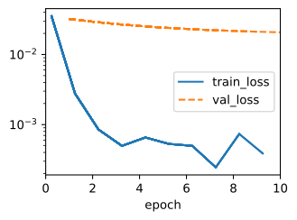
L2 norm of w: 0.011407211422920227

A framework’s weight_decay adds \lambda\mathbf{w} to the gradient; the scratch penalty added \tfrac{\lambda}{2}\|\mathbf{w}\|^2 to the loss. Converged norms need not match exactly, only the effect.

The adaptive-optimizer reading: AdamW

Beyond linear models

Inside an Adam-style update each coordinate gets its own step size, so folding the penalty into the gradient rescales it per coordinate: it stops being uniform shrinkage.

Decoupling the decay from the adaptive step restores the intent of plain 1-\eta\lambda shrinkage. This is AdamW, a default for training large models.

For deep networks we simply apply the same decay to every layer’s weights: a simple, effective default.

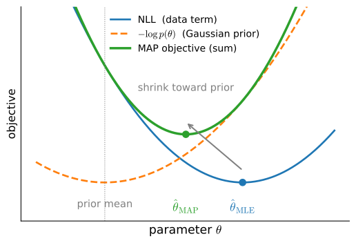
The Bayesian reading: a prior on the weights

Beyond linear models

Put a zero-mean Gaussian prior on \mathbf{w}:

\mathbf{w}\sim\mathcal{N}(\mathbf{0},\lambda^{-1}\mathbf{I}) \;\Rightarrow\; -\log p(\mathbf{w}) = \tfrac{\lambda}{2}\|\mathbf{w}\|^2 + \textrm{const}.

Add it to the Gaussian-noise NLL from the linear-regression section:

\underbrace{-\log p(\mathbf{y}\mid\mathbf{X},\mathbf{w})}_{\textrm{MLE: }\,\frac{1}{2\sigma^2}\sum(\hat{y}-y)^2} \;\; \underbrace{-\log p(\mathbf{w})}_{=\,\frac{\lambda}{2}\|\mathbf{w}\|^2} \;\Rightarrow\; \textrm{MAP} = \textrm{ridge}.

MAP = MLE + a prior. The linear-regression section got squared loss from Gaussian noise; weight decay adds a Gaussian prior on \mathbf{w}, with \lambda the prior precision.

A Gaussian prior centred at zero pulls the maximum-likelihood estimate back toward the origin.

Summary

Wrap-up

• Weight decay = original loss +\ \tfrac{\lambda}{2}\|\mathbf{w}\|_2^2; per step it shrinks the weights by 1 - \eta\lambda before the data update.
• Geometry: ridge shrinks (round ball), lasso selects (pointed diamond).
• Spectral view: each direction damped by d_j^2/(d_j^2+\tilde\lambda); the 200-knob model ran at \textrm{df} \approx 15 effective parameters, a continuous dial tuned on a validation set.

• The 20{\times}200 rig: \lambda=0 memorizes; \lambda=3 trades training error for a falling validation loss.
• Frameworks expose decay in the optimizer (or layer / gradient transform).
• Same idea scales up: AdamW for big models, a Gaussian prior in disguise.