Softmax Regression
Dive into Deep Learning · §3.1
From scores to probabilities to a loss
one-hot labels · the softmax · linear decision boundaries · cross-entropy.
From how much to which class
Motivation
Regression answered how much? Classification asks which category?: spam or inbox, cat or dog or chicken.
- A linear layer still produces one score per class.
- The softmax turns those scores into a probability distribution.
- Cross-entropy measures how surprised that distribution is by the truth.
The whole section is one pipeline: scores \to probabilities \to loss.
01
Labels & the Linear Model
one-hot encoding and one score per class
One-hot: a label is a vector
Labels
Classes have no natural order, so we do not encode “cat, chicken, dog” as 1, 2, 3. Instead each label is a one-hot vector, a 1 in its class slot and 0 elsewhere:
y \in \{(1,0,0),\ (0,1,0),\ (0,0,1)\}.
This puts the label in the same space as a probability vector, so we can compare prediction and truth coordinate by coordinate.
One affine function per class
Linear Model
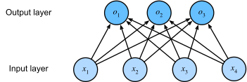
With 4 features and 3 classes we need a 3\times4 weight matrix and a bias per class, packed into a single fully connected layer:
\mathbf{o} = \mathbf{W}\mathbf{x} + \mathbf{b}.
Each output o_i depends on every input. These raw scores are the logits; they are not yet probabilities.
Why not just regress onto the labels?
Linear Model
We could try to fit \mathbf{o} directly to the one-hot \mathbf{y}. But raw logits make poor probabilities:
Nothing forces o_i \ge 0, and nothing forces \sum_i o_i = 1.
A linear score can run past 1 or below 0, so a “probability” of buying a mansion could exceed 100%. We need a map that squishes any score vector onto valid probabilities.
02
The Softmax
exponentiate, then normalize
The softmax: squish scores to probabilities
The Softmax
Exponentiate each score (now nonnegative), then divide by the row sum (now sums to 1):
\hat{y}_i = \mathrm{softmax}(\mathbf{o})_i = \frac{\exp(o_i)}{\sum_j \exp(o_j)}.
The denominator \sum_j \exp(o_j) is the partition function, the same normalizer Boltzmann used for energy states in a gas, with energy playing the role of (negative) score.
Softmax keeps the ranking
The Softmax
The exponential is monotone, so the largest score stays the largest probability:
\operatorname*{argmax}_j \hat{y}_j = \operatorname*{argmax}_j o_j.
So to predict a class we never need to compute the softmax; we read off the biggest logit. The softmax matters for the loss, not the decision.
Temperature controls distribution sharpness
The Softmax · temperature
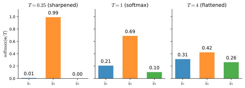
Boltzmann weighted energy states by \exp(-E/kT); for us, replace \mathrm{softmax}(\mathbf{o}) by \mathrm{softmax}(\mathbf{o}/T). The same three scores, at three temperatures:
![]()
Cooling (T=0.25) piles the mass on the top class; T=1 is plain softmax; heating (T=4) approaches uniform. Same scores \mathbf{o}=(1.0, 2.2, 0.3), same ordering, in every panel.
1/T scales every logit alike, so the ranking never changes: only the confidence does. The calibration discussion below returns to this parameter.
Softmax from randomized utility
The Softmax · origins
Another route to probabilities: perturb each score and report the winner, y = \operatorname*{argmax}_i\,(o_i + \epsilon_i).
- Gaussian noise gives the (multinomial) probit model (Fechner, 1860): appealing, but no closed form and a harder optimization.
- Gumbel noise gives exactly \mathrm{softmax}(\mathbf{o}), the Gumbel-max trick (exercise 9), and scaling the noise by T samples from \mathrm{softmax}(\mathbf{o}/T).
So the softmax is a smoothed argmax, with temperature the amount of smoothing.
Only differences of logits matter
The Softmax · invariance
Add the same constant c to every logit. Numerator and denominator both pick up a factor \exp(c), which cancels:
\mathrm{softmax}(\mathbf{o} + c\mathbf{1}) = \mathrm{softmax}(\mathbf{o}).
The scores carry one redundant degree of freedom: we may pin o_q \equiv 0 without changing any prediction. (This same shift, with c = -\max_k o_k, is the trick that makes the computation numerically stable.)
Two classes: softmax is the sigmoid
The Softmax · special case
With q = 2, only the logit gap o = o_1 - o_2 survives:
\hat{y}_1 = \frac{\exp(o_1)}{\exp(o_1)+\exp(o_2)} = \frac{1}{1 + \exp(-o)} = \sigma(o).
Binary logistic regression is just softmax regression with the redundant logit removed: the same model, one class folded away.
The decision boundaries are always straight lines
The Softmax · geometry
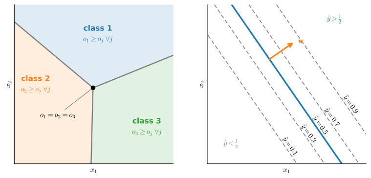
The predicted class is \operatorname{argmax}_j o_j with each o_j affine, so class j wins where finitely many linear inequalities o_j \ge o_k hold: a convex polyhedron per class.
![]()
Left: three convex regions, straight boundaries at the ties o_i = o_j. Right: two classes, parallel level lines of \sigma(o), perpendicular to \mathbf{w}.
Softmax changes the probabilities, but the decision boundaries remain linear. The from-scratch experiment measures the resulting model on images (the softmax-from-scratch section).
03
Cross-Entropy Loss
maximum likelihood over discrete labels
Maximum likelihood becomes a sum of losses
Loss
The model reads \hat{\mathbf{y}} as conditional class probabilities. Over an i.i.d. dataset the likelihood factorizes; taking -\log turns the product into a sum:
-\log P(\mathbf{Y}\mid\mathbf{X}) = \sum_{i=1}^n l\bigl(\mathbf{y}^{(i)}, \hat{\mathbf{y}}^{(i)}\bigr).
Minimizing this negative log-likelihood applies the same principle used to derive squared error, now for discrete categories.
The cross-entropy loss
Loss
For a one-hot label \mathbf{y} the per-example loss keeps only the true class’s term:
l(\mathbf{y}, \hat{\mathbf{y}}) = -\sum_{j=1}^q y_j \log \hat{y}_j = -\log \hat{y}_{\text{true}}.
It is \ge 0, and 0 only with certainty on the right class, which finite logits can never quite reach. Predict the truth with high confidence and the loss is small; predict it with near-zero probability and the loss becomes large.
The gradient: prediction minus truth
Loss · gradient
Substitute the softmax into the loss and it collapses to a log-partition term minus a linear term, l = g(\mathbf{o}) - \mathbf{y}^\top\mathbf{o} with g(\mathbf{o}) = \log\sum_k \exp(o_k). Differentiate:
\partial_{o_j}\, l(\mathbf{y}, \hat{\mathbf{y}}) = \mathrm{softmax}(\mathbf{o})_j - y_j = \hat{y}_j - y_j.
The gradient is the residual, predicted probability minus observed label, exactly as in linear regression. In an exponential-family model with canonical natural parameters, the general form is expected sufficient statistics minus observed sufficient statistics; here those statistics are class indicators.
Why
Loss · information theory
Entropy H[P] = \sum_j -P(j)\log P(j) is the average number of nats needed to encode draws from P (natural log throughout). Cross-entropy H(P, Q) = \sum_j -P(j)\log Q(j) is the cost of coding P’s draws with a wrong model Q.
Our loss is H(\mathbf{y}, \hat{\mathbf{y}}).
So minimizing it does two equivalent things: it maximizes likelihood and it minimizes excess coding cost relative to the target distribution.
Confidence is not calibrated probability
Loss · a modern caveat
The loss keeps rewarding confidence even after the decision is right, nudging 0.51 \to 0.99. So do not read the outputs at face value: a cross-entropy-trained network is generally not calibrated: a reported 0.9 does not mean right 90\% of the time. Modern deep nets are systematically overconfident :cite:Guo.Pleiss.Sun.Weinberger.2017.
The fix is the dial we already hold: temperature scaling divides the logits by one learned T > 0 before the softmax: Boltzmann’s T, relearned post hoc.
Because 1/T scales every logit alike, the ranking (hence the \arg\max, hence the accuracy) is untouched; only the confidences sharpen (T<1) or soften (T>1). Exercise 8 develops this.
04
Two Faces of the Scores
the same logits drive training and evaluation
One score vector, two jobs
Synthesis
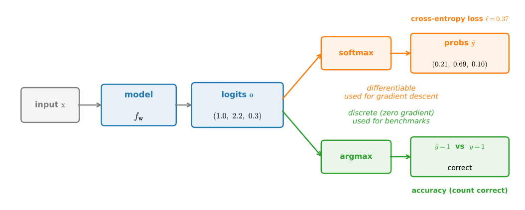
A single forward pass produces logits \mathbf{o}; the picture forks.
- Train: softmax \to probabilities \to cross-entropy. Smooth and differentiable, so gradient descent minimizes it.
- Evaluate: \arg\max \to a hard class \to accuracy. Discrete with zero gradient, the number we report.
Both branches read the same scores.
Summary
Wrap-up
- One-hot labels live in probability space; a linear layer emits one logit per class.
- Softmax \hat{y}_i \propto \exp(o_i) is a smoothed argmax (Gumbel noise makes that exact); temperature T dials argmax \leftrightarrow uniform without changing the ranking.
- Only logit differences matter; two classes recover the sigmoid; decision boundaries are straight lines, always.
- Cross-entropy = -\log \hat{y}_{\text{true}} is the negative log-likelihood, equivalently a code length.
- Its gradient is the residual \hat{\mathbf{y}} - \mathbf{y}: convex, cheap, shared by all exponential families.
- Confidence \neq calibrated probability; temperature scaling recalibrates without touching accuracy.