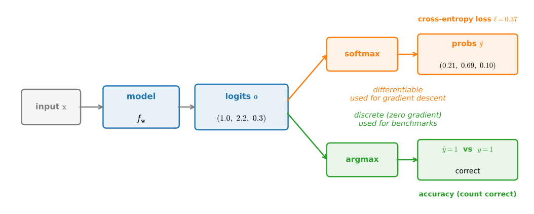
Three steps: exponentiate every score, sum across the class axis, divide each row by its total:
def softmax(X): X_exp = d2l.exp(X) partition = d2l.reduce_sum(X_exp, 1, keepdims=True)return X_exp / partition # The broadcasting mechanism is applied here
Naive expoverflows for large logits. This direct implementation exposes the formula but is numerically unstable. The stable fix arrives in the concise-softmax-regression section.
The output is a real distribution
The Softmax
Feed in any matrix: every entry becomes non-negative and each row sums to 1, exactly what a probability distribution over classes requires:
X = jax.random.uniform(d2l.get_key(), (2, 5))X_prob = softmax(X)X_prob, d2l.reduce_sum(X_prob, 1)
A single logit of 1000 sends \exp to infinity in float32, so the max entry becomes \infty/\infty=NaN (and the rest underflow to 0), making the row invalid. The framework’s softmax shifts by the row maximum first and stays finite on the identical input:
A NaN propagates through downstream gradients. The concise-softmax-regression section derives the fix (fuse softmax and log via log-sum-exp) and shows the frameworks already ship it.
02
The Model
one linear layer, ten logits
Parameters: a 784×10 weight matrix
The Model
Each 28\times28 image flattens to a length-784 vector; with 10 classes the weights are a 784\times10 matrix W plus a length-10 bias b. Initialize W with Gaussian noise, b with zeros:
The model is one expression: reshape the batch to rows of 784, apply the affine map \mathbf{X}\mathbf{W}+\mathbf{b}, then softmax into per-class probabilities:
Minimizing cross-entropy maximizes the log-likelihood of the correct labels. It distinguishes correct-class probabilities of 0.51\to0.99 even when the hard decision is unchanged.
Average over the batch
Cross-Entropy Loss
Take the negative log of each selected probability, then average. A tiny clip keeps the log finite when a probability underflows to 0:
def cross_entropy(y_hat, y):# Tiny clip to keep log finite when softmax outputs underflow to 0. p = jnp.clip(jnp.take_along_axis(y_hat, jnp.expand_dims(y, -1), axis=1).squeeze(-1), min=1e-12)return-d2l.reduce_mean(d2l.log(p))cross_entropy(y_hat, y)
Array(1.4978662, dtype=float32)
The clip only masks \log 0; it does not fix the upstream overflow, and it silently kills the gradient on any clamped entry. The concise-softmax-regression section derives the stable fused loss.
Register it as the loss
Cross-Entropy Loss
Attach cross_entropy as the model’s loss, and every reused training utility now knows how to optimize this classifier:
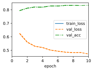
Ten epochs of minibatch SGD on Fashion-MNIST. The inherited Classifier runs the validation loop and plots train/validation loss alongside validation accuracy, no extra code:
data = d2l.FashionMNIST(batch_size=256)model = SoftmaxRegressionScratch(num_inputs=784, num_outputs=10, lr=0.1)trainer = d2l.Trainer(max_epochs=10)trainer.fit(model, data)
Predictions on a validation batch
Prediction
Take the argmax of the model’s outputs over a fresh validation batch, one predicted class per image:
X, y =next(iter(data.val_dataloader()))preds = d2l.argmax(model(X), axis=1)preds.shape
(256,)
Inspect misclassified examples
Prediction
We inspect the errors to identify recurring class confusions. Tile the misclassified images, each captioned true / predicted:
wrong = d2l.astype(preds, y.dtype) != yX, y, preds = X[wrong], y[wrong], preds[wrong]labels = [a+'\n'+b for a, b inzip( data.text_labels(y), data.text_labels(preds))]data.visualize([X, y], labels=labels)
Validation accuracy of the linear model
Prediction
Sweep the whole validation set and average the per-example correct flags returned by accuracy(..., averaged=False): the overall test accuracy lands at roughly 82–83% in the displayed run, matching the validation curve above.
The next slide resolves this aggregate accuracy into class-specific errors.
The confusion matrix identifies two error groups
Prediction · the confusion matrix
Accumulate a 10\times 10 count matrix over the validation set (the base-classification section’s confusion matrix), normalize each column, and the errors concentrate in a few groups:
Upper-body garments (t-shirt, pullover, dress, coat, shirt) trade errors almost exclusively among themselves; the shirt column has the largest off-diagonal mass, often assigned to t-shirt, pullover, or coat.
Footwear (sandal, sneaker, ankle boot) forms a second, smaller cluster.
Trousers and bags have predominantly diagonal entries in this run.
Same outline, same mass distribution → indistinguishable to a model that can only weigh pixels linearly.
What the linear model cannot represent
Model capacity
A linear classifier draws straight decision boundaries: as shown in the softmax-regression section. In pixel space shirts and pullovers overlap, and no hyperplane separates them.
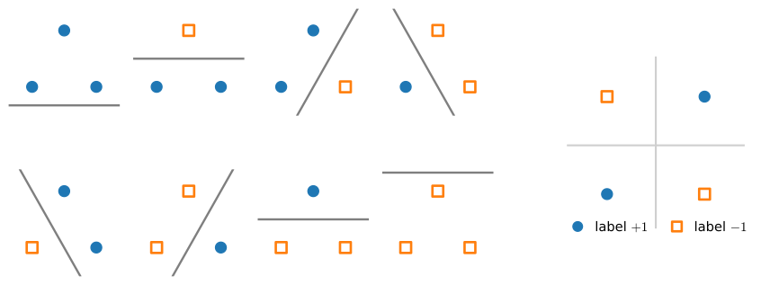
The capacity of lines is finite: in the plane a line can shatter 3 points in general position but cannot realize the 4-point XOR labeling (the generalization-in- classification section makes this precise). A single hidden layer (the multilayer-perceptrons chapter) can represent nonlinear decision boundaries.
Recap
Wrap-up
Softmax = exp, row-sum, divide → a probability distribution over classes.
Cross-entropy = -\log \hat{y}_{\text{true}}, averaged over the batch: the negative log-likelihood used here.
Model = flatten → one linear layer (784\times10) → softmax.
Training reuses the regression Trainer; Classifier adds accuracy reporting through the base class.
This run reaches 82–83%; its confusion matrix concentrates errors among visually similar upper-body garments and, to a lesser extent, footwear.
exp(1000) = NaN: the naive softmax is fragile and clipping does not address the overflow; the concise-softmax-regression section derives the stable approach.