key = jax.random.PRNGKey(0)
mix = d2l.GaussianMixture(means=[[-2.5, -1.5], [2.5, -1.5], [0.0, 2.5]],
                          weights=[0.5, 0.3, 0.2], std=0.5)
key, k1, k2 = jax.random.split(key, 3)
data, test = mix.sample(k1, 2000), mix.sample(k2, 2000)

class ScoreNet(nnx.Module):
    """A two-dimensional score model: a multilayer perceptron with two outputs."""
    def __init__(self, hidden=128, rngs=None):
        self.h1 = nnx.Linear(2, hidden, rngs=rngs)
        self.h2 = nnx.Linear(hidden, hidden, rngs=rngs)
        self.out = nnx.Linear(hidden, 2, rngs=rngs)

    def __call__(self, x):
        return self.out(nnx.silu(self.h2(nnx.silu(self.h1(x)))))

def fisher_divergence(score, x):
    """0.5 E||s(x) - grad log p(x)||^2 on the given points."""
    return float(0.5 * ((score(x) - mix.score(x)) ** 2).sum(1).mean())

def score_matching_loss(score, x):
    """Hyvarinen's objective E[0.5 ||s||^2 + tr(ds/dx)], trace by autodiff."""
    s = score(x)
    f = lambda q: score(q[None])[0]  # the field at a single point, for its Jacobian
    trace = jax.vmap(lambda q: jnp.trace(jax.jacfwd(f)(q)))(x)
    return (0.5 * (s ** 2).sum(1) + trace).mean()

def objective_on(score, x, chunks=10):  # average over a large sample
    return float(sum(score_matching_loss(score, c)
                     for c in jnp.array_split(x, chunks)) / chunks)

key, subkey = jax.random.split(key)
big = mix.sample(subkey, 200_000)
const = float(0.5 * (mix.score(big) ** 2).sum(1).mean())
objective = objective_on(mix.score, big)
print(f'objective at the true score: {objective:.3f}, '
f'constant: {const:.3f}, sum: {objective + const:.3f}')Score Matching
Dive into Deep Learning · §17.3
Score matching
the score needs no normalizer · the Fisher divergence · Hyvärinen’s identity · sliced estimation
The Score Is the Input Gradient of the Log-Density
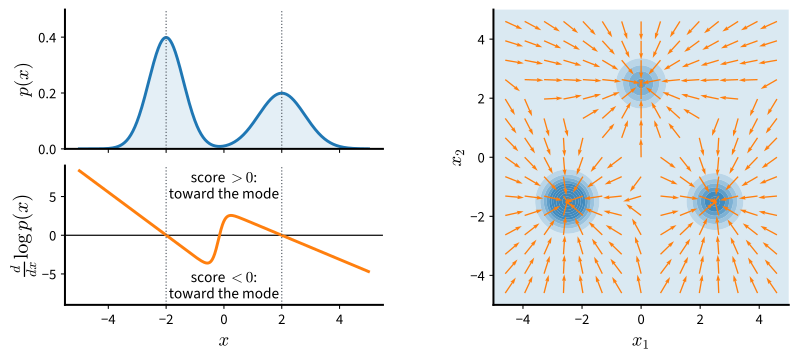
\nabla_{\mathbf{x}} \log p(\mathbf{x}) : \mathbb{R}^d \to \mathbb{R}^d, \qquad \nabla_{\mathbf{x}} \log p_{\boldsymbol{\theta}}(\mathbf{x}) = -\nabla_{\mathbf{x}} E_{\boldsymbol{\theta}}(\mathbf{x})
A vector field pointing toward the modes, and for an energy-based model, free of Z(\boldsymbol{\theta}).
Match Score Fields, Not Densities
J_{\textrm{ESM}}(\boldsymbol{\theta}) = \tfrac{1}{2}\, \mathbb{E}_{\mathbf{x} \sim p} \big\| \mathbf{s}_{\boldsymbol{\theta}}(\mathbf{x}) - \nabla_{\mathbf{x}} \log p(\mathbf{x}) \big\|^2
- zero exactly when the fields agree on the data;
- no partition function anywhere;
- but \nabla_{\mathbf{x}} \log p is the data score, which we do not have.
Hyvärinen’s Identity Moves the Derivative onto the Model
Integration by parts on the cross term, in one dimension:
-\int s_{\boldsymbol{\theta}}\, p'\, dx = -\big[ s_{\boldsymbol{\theta}}\, p \big]_{-\infty}^{\infty} + \int s_{\boldsymbol{\theta}}'\, p\, dx = \mathbb{E}_p[s_{\boldsymbol{\theta}}']
J_{\textrm{ESM}}(\boldsymbol{\theta}) = \mathbb{E}_{\mathbf{x} \sim p} \Big[ \tfrac{1}{2} \| \mathbf{s}_{\boldsymbol{\theta}} \|^2 + \operatorname{tr}\big( \nabla_{\mathbf{x}} \mathbf{s}_{\boldsymbol{\theta}} \big) \Big] + \textrm{const}
Only the model appears under the expectation: training needs data alone.
The Identity, Checked Numerically
At the true score the Fisher divergence is zero, so the objective must equal minus the constant:
objective at the true score: -4.005, constant: 3.994, sum: -0.011Two large terms of opposite sign cancel; that cancellation is also why the objective is noisy on small samples.
Sliced Score Matching Estimates the Trace by Projection
J_{\textrm{SSM}}(\boldsymbol{\theta}) = \mathbb{E}_{\mathbf{v}}\, \mathbb{E}_{\mathbf{x} \sim p} \Big[ \mathbf{v}^\top \nabla_{\mathbf{x}} \mathbf{s}_{\boldsymbol{\theta}}(\mathbf{x})\, \mathbf{v} + \tfrac{1}{2} \big( \mathbf{v}^\top \mathbf{s}_{\boldsymbol{\theta}}(\mathbf{x}) \big)^2 \Big]
- the trace costs d derivative passes; a directional derivative costs one;
- unbiased when \mathbb{E}[\mathbf{v}\mathbf{v}^\top] = I, at the cost of variance;
- comparable fit after the same number of updates on the running example.
Both Estimators Fit the Field Where the Data Are
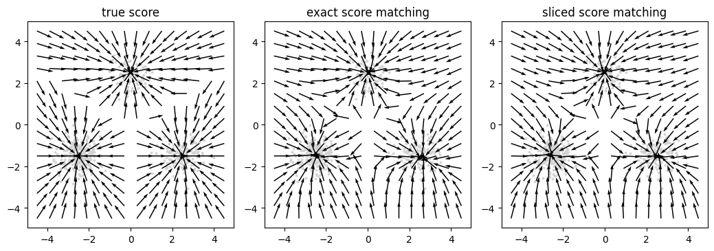
Near the modes the learned fields agree with the truth; in the corners and between the modes, nothing constrained them.
Accuracy Follows the Data Density
axis = jnp.linspace(-5, 5, 41)
grid = jnp.stack(jnp.meshgrid(axis, axis, indexing='ij'), -1).reshape(-1, 2)
true_s, log_p = mix.score(grid), mix.log_prob(grid)
err = ((score_exact(grid) - true_s) ** 2).sum(1)
print(f'{"log density":>13} {"grid points":>12} {"relative score error":>21}')
for lo, hi in ((-2, 0), (-4, -2), (-8, -4), (-16, -8), (-40, -16)):
    m = (log_p >= lo) & (log_p < hi)
    rel = err[m].mean() / (true_s[m] ** 2).sum(1).mean()
    print(f'[{lo:>4}, {hi:>4}) {int(m.sum()):>12d} {rel:>21.3f}')
log density grid points relative score error
[ -2, 0) 30 0.068
[ -4, -2) 145 0.024
[ -8, -4) 308 0.034
[ -16, -8) 557 0.154
[ -40, -16) 547 0.134Under ten percent where the data are; ten to twenty percent about three orders of magnitude down in density. Samplers that start from noise begin where the estimate is least accurate.
Recap
- Score = \nabla_{\mathbf{x}} \log p: for an energy-based model, -\nabla_{\mathbf{x}} E_{\boldsymbol{\theta}}, no Z.
- Fisher divergence measures field mismatch; Hyvärinen’s identity makes it computable from data alone via \tfrac12 \|\mathbf{s}\|^2 + \operatorname{tr}(\nabla \mathbf{s}).
- The trace scales with d; sliced score matching replaces it by a random projection.
- The fit is accurate only where the data are. Next: perturb the data with noise, which removes the Jacobian and fills the empty regions.