K = 64
axis = jnp.linspace(-6, 6, K)
for d in (1, 2, 3):
    energy_d = make_energy(d)
    pts = jnp.stack(jnp.meshgrid(*([axis] * d), indexing='ij'),
                    -1).reshape(-1, d)
    log_Z = (jax.nn.logsumexp(-energy_d(pts), 0)
             + d * math.log(axis[1] - axis[0]))
    print(f'd = {d}: {len(pts):>7d} energy evaluations, log Z = {log_Z:7.3f}')
for d in (10, 784):
print(f'd = {d}: {K}^{d} = 10^{d * math.log10(K):.0f} energy evaluations')The Limits of GANs and Energy-Based Models
Dive into Deep Learning · §17.1
The limits of GANs and energy-based models
what the adversarial game leaves unsolved · densities from nearly any network · the price of the partition function
Adversarial Training Has the Right Fixed Point but Four Problems
Against the optimal discriminator, the generator’s objective is minimized at p_g = p_{\textrm{data}}, yet
- simultaneous gradient steps can circle or spiral away from the equilibrium (the Dirac-GAN);
- with a perfect discriminator, the saturating loss has no gradient and the non-saturating one is noisy;
- mode-dropping minima exist, and the fixes are empirical;
- there is no density to evaluate: no held-out likelihood, no likelihood-based anomaly score.
This chapter keeps the flexible network and restores the density.
Normalization Is the Constraint That Makes Learning Meaningful
Nonnegativity is free: \exp(f_{\boldsymbol{\theta}}(\mathbf{x})) works for any network.
Sum-to-one is not: raising the density on training points must lower it elsewhere.
Earlier families pay for normalization:
- products of conditionals (autoregressive),
- mixtures of normalized components, with a tractable sum or a lower bound (latent variables),
- bijections with tractable Jacobians (flows).
An Energy-Based Model Normalizes Explicitly
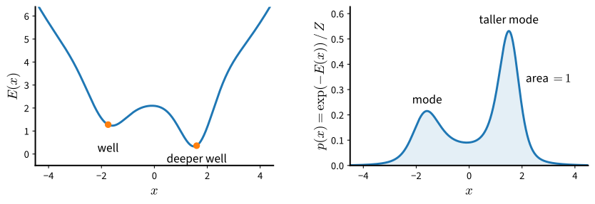
p_{\boldsymbol{\theta}}(\mathbf{x}) = \frac{\exp(-E_{\boldsymbol{\theta}}(\mathbf{x}))}{Z(\boldsymbol{\theta})}, \qquad Z(\boldsymbol{\theta}) = \int \exp(-E_{\boldsymbol{\theta}}(\mathbf{x}))\, d\mathbf{x}
Any scalar network with integrable \exp(-E_{\boldsymbol{\theta}}) is an energy; the whole difficulty sits in the one number Z.
Without the Normalizer: Ratios, Rankings, Minimization
\frac{p_{\boldsymbol{\theta}}(\mathbf{x})}{p_{\boldsymbol{\theta}}(\mathbf{x}')} = \exp\big(E_{\boldsymbol{\theta}}(\mathbf{x}') - E_{\boldsymbol{\theta}}(\mathbf{x})\big)
- compare or rank inputs; flag an input far less probable than typical data;
- denoise by minimizing the energy near the corrupted input; impute by minimizing it over the missing coordinates;
- predict with a conditional energy E(\mathbf{x}, y) by minimizing over y.
Not available: the likelihood, and a sample.
Quadrature Costs K^d Evaluations
d = 1:      64 energy evaluations, log Z =   2.315
d = 2:    4096 energy evaluations, log Z =   3.643
d = 3:  262144 energy evaluations, log Z =   4.184
d = 10: 64^10 = 10^18 energy evaluations
d = 784: 64^784 = 10^1416 energy evaluations
Three dimensions: a quarter of a million points. Ten: a billion billion. An image: an exponent above a thousand.
Importance Sampling Is Unbiased but Degrades with Dimension
Target \mathcal{N}(\mathbf{1}, I), proposal \mathcal{N}(\mathbf{0}, I): one standard deviation apart per coordinate, and the relative standard error of \hat Z is exactly \sqrt{(e^d - 1)/n}.
key = jax.random.PRNGKey(1)
n = 100_000
print(f'{"d":>3} {"estimate / Z":>13} {"predicted rel. std. error":>26} '
      f'{"effective samples":>18}')
for d in (1, 2, 4, 8, 16, 32):
    key, subkey = jax.random.split(key)
    x = jax.random.normal(subkey, (n, d))      # proposal q = N(0, I)
    log_w = x.sum(1) - d / 2                   # log (w / Z)
    log_sum = jax.nn.logsumexp(log_w, 0)
    estimate = jnp.exp(log_sum - math.log(n))
    ess = jnp.exp(2 * log_sum - jax.nn.logsumexp(2 * log_w, 0))
    print(f'{d:>3} {estimate:>13.3f} {math.sqrt((math.exp(d) - 1) / n):>26.3g} '
          f'{ess:>18.1f}')
d estimate / Z predicted rel. std. error effective samples
1 1.000 0.00415 37568.7
2 0.997 0.00799 14351.7
4 0.985 0.0232 1425.4
8 1.003 0.173 145.8
16 1.088 9.43 6.0
32 0.079 2.81e+04 10.5By d = 16 a hundred thousand draws carry under a hundred effective samples.
Recap
- GANs: unrestricted generator, no density to evaluate; a game that may cycle, saturate, or drop modes.
- Energy-based models: p_{\boldsymbol{\theta}} = \exp(-E_{\boldsymbol{\theta}}) / Z(\boldsymbol{\theta}) with any network whose \exp(-E_{\boldsymbol{\theta}}) is integrable; ratios and minimization are free, likelihood and samples are not.
- Z by grid: K^d evaluations. Z by importance sampling from a proposal one standard deviation off per coordinate: relative error grows like e^{d/2}.
- Next: the maximum-likelihood gradient needs samples from the model, not Z itself.