Sampling with Langevin Dynamics

Dive into Deep Learning · §17.5

Sampling with Langevin dynamics
gradient ascent plus noise · exact in the limit, stuck in practice · the smoothing trade-off

Langevin Dynamics: Follow the Score, Add Noise

\mathbf{x}_{k+1} = \mathbf{x}_k + \frac{\alpha}{2}\, \nabla_{\mathbf{x}} \log p(\mathbf{x}_k) + \sqrt{\alpha}\, \boldsymbol{\xi}_k, \qquad \boldsymbol{\xi}_k \sim \mathcal{N}(\mathbf{0}, I)

  • the Euler–Maruyama step of d\mathbf{X} = \tfrac12 \nabla \log p\, dt + d\mathbf{W}, for which p is stationary;
  • a discretization bias for the discrete chain that vanishes with \alpha; a Metropolis test removes it;
  • needs only the score: plug in \mathbf{s}_{\boldsymbol{\theta}}.

With the Exact Score: Right Modes, Wrong Weights

key, k1, k2 = jax.random.split(key, 3)
x_init = 3 * jax.random.normal(k1, (2000, 2))
true_score = TrueScore()
print(f'target (2000 samples of the mixture): {summarize(data)}')
for steps in (200, 2000):
    key, subkey = jax.random.split(key)
    print(f'true score, {steps:>4d} steps:   '
          f'{summarize(langevin(true_score, x_init, subkey, steps, 0.05))}')
x_one = mix.means[0] + mix.std * jax.random.normal(k2, (2000, 2))
key, subkey = jax.random.split(key)
print(f'true score, start in mode 1: '
      f'{summarize(langevin(true_score, x_one, subkey, 2000, 0.05))}')
target (2000 samples of the mixture): mode weights [0.517, 0.296, 0.187], spread 0.46, stray 0.011
true score,  200 steps:   mode weights [0.318, 0.325, 0.358], spread 0.48, stray 0.019
true score, 2000 steps:   mode weights [0.32, 0.327, 0.354], spread 0.51, stray 0.020
true score, start in mode 1: mode weights [0.999, 0.001, 0.001], spread 0.50, stray 0.012

Each mode is reproduced to within the step-size bias; the weights are those of the initialization, after two hundred steps and after two thousand. Crossing a valley whose floor is five standard deviations from either mode takes far longer than any run.

Chains Fall into a Basin and Stay

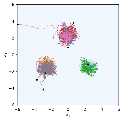
Eight chains started from noise: a quick descent, then a wander inside one basin. The gradient does not cure slow mixing.

A Learned Score Is Consulted Where It Is Worst
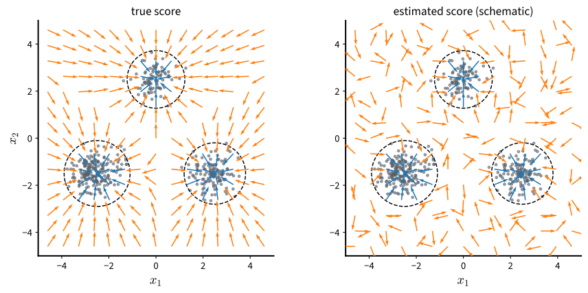
A chain from noise starts outside the dashed line, where the estimate had no data to fit. For images, almost all of pixel space is such a region.

Smoothing Fixes Mixing and Blurs the Samples
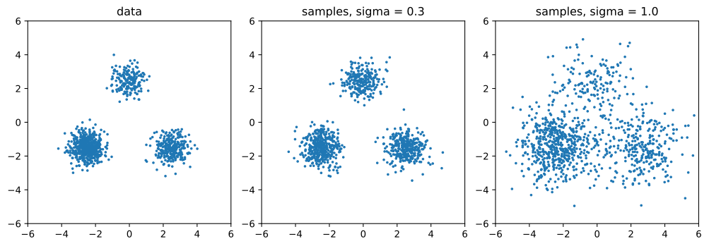
At \sigma = 1 the weights are right and the samples are blurred; at \sigma = 0.3 the samples are sharp and the weights are wrong.

Recap

  • Langevin dynamics turns a score into a sampler; correctness is asymptotic.
  • Failure one: separated modes are not crossed, so weights reflect the start.
  • Failure two: a learned score is unreliable in the empty regions the chain must traverse.
  • At large \sigma, Gaussian smoothing largely removes both but samples the blurred distribution. Next: a ladder of noise levels.