def true_velocity(x, t):  # the linear-path velocity, from the closed-form score
    return x / t + (1 - t) / t * mix.score(x, scale=t, sigma=1 - t)

print(f'{"t":>4} {"E||v - u||^2":>13} {"E||u||^2":>9}')
for t in (0.2, 0.5, 0.8, 0.95):
    key, subkey = jax.random.split(key)
    x_t = (1 - t) * jax.random.normal(subkey, test.shape) + t * test
    u = true_velocity(x_t, t)
    v = velocity(x_t, jnp.full((len(test),), t))
print(f'{t:>4} {((v - u) ** 2).sum(1).mean():>13.3f} {(u ** 2).sum(1).mean():>9.3f}')Flow Matching and Its Relation to Diffusion
Dive into Deep Learning · §17.10
Flow matching and its relation to diffusion
paths and velocity fields · conditional flow matching · one dictionary for scores and velocities
Prescribe the Path, Learn the Velocity
\frac{d}{dt} \mathbf{x}_t = \mathbf{u}_t(\mathbf{x}_t),\qquad \mathbf{x}_0 \sim \mathcal{N}(\mathbf{0}, I),\qquad \mathbf{x}_1 \sim p_{\textrm{data}}
- a velocity field generates the path when mass moves with it (continuity equation);
- sampling is numerical integration, noise to data;
- the marginal field is unknown, like the data score.
Conditional Flow Matching on Straight Segments
\mathbf{x}_t = (1 - t)\, \mathbf{x}_0 + t\, \mathbf{x}_1,\qquad \mathcal{L}_{\textrm{CFM}} = \mathbb{E}\, \big\| \mathbf{v}_{\boldsymbol{\theta}}(\mathbf{x}_t, t) - (\mathbf{x}_1 - \mathbf{x}_0) \big\|^2
- the marginal velocity is the posterior mean of the segment direction;
- regressing onto it has the same minimizer (the regression lemma again);
- draw noise, draw data, interpolate, regress.
Two Gaussian Paths from Noise to Data
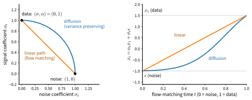
Same endpoints, different geometry: diffusion moves along the circle \alpha^2 + \sigma^2 = 1, flow matching along the line \alpha + \sigma = 1.
The Score–Velocity Dictionary
\mathbf{u}_t(\mathbf{x}) = \frac{\dot{\alpha}_t}{\alpha_t}\, \mathbf{x} - \Big( \sigma_t \dot{\sigma}_t - \sigma_t^2\, \frac{\dot{\alpha}_t}{\alpha_t} \Big) \nabla_{\mathbf{x}} \log p_t(\mathbf{x})
- both sides are affine in the posterior mean \hat{\mathbf{x}}_1 (Tweedie);
- a trained noise predictor is therefore a velocity field: DDIM integrates it;
- linear path: \mathbf{u}_t = \mathbf{x}/t + \tfrac{1-t}{t}\, \nabla \log p_t.
The Dictionary, Checked on the Mixture
   t  E||v - u||^2  E||u||^2
 0.2         0.104     1.068
 0.5         0.169     7.708
 0.8         0.040     8.038
0.95         0.130     8.378
Learned velocity against the velocity computed from the closed-form score: a few percent apart in mean square for t \geq 0.5, with no score learned and no velocity in the formula.
Euler Steps and Curvature
def euler_sample(field, x, steps, record=False):
    trajectory = [x]
    for k in range(steps):
        x = x + field(x, jnp.full((len(x),), k / steps)) / steps
        trajectory.append(x)
    return (x, jnp.stack(trajectory)) if record else x

def summarize(x):
    d2 = ((x[:, None, :] - mix.means[None]) ** 2).sum(-1)
    weights = [round(float(w), 3) for w in
               jnp.bincount(d2.argmin(1), length=3) / len(x)]
    nearest = d2.min(1)
    inside = nearest < (3 * mix.std) ** 2
    return (f'mode weights {weights}, spread {nearest[inside].mean():.2f}, '
            f'stray {1 - inside.mean():.3f}')

def curvature(trajectory):  # path length over chord length, minus one
    length = jnp.linalg.norm(trajectory[1:] - trajectory[:-1], axis=2).sum(0)
    chord = jnp.linalg.norm(trajectory[-1] - trajectory[0], axis=1)
    return (length / chord - 1).mean()

key, subkey = jax.random.split(key)
x0 = jax.random.normal(subkey, (2000, 2))
print(f'target (2000 samples of the mixture): {summarize(data)}')
for steps in (100, 10, 4, 2):
    print(f'learned field, {steps:>3d} Euler steps: {summarize(euler_sample(velocity, x0, steps))}')
exact = lambda x, t: true_velocity(x, jnp.maximum(t[0], 1e-3))  # avoid t = 0
print(f'exact field,   100 Euler steps: {summarize(euler_sample(exact, x0, 100))}')
_, path = euler_sample(velocity, x0, 100, record=True)
print(f'curvature of the learned flow: {curvature(path):.3f}')
target (2000 samples of the mixture): mode weights [0.517, 0.296, 0.187], spread 0.46, stray 0.011
learned field, 100 Euler steps: mode weights [0.523, 0.291, 0.187], spread 0.47, stray 0.038
learned field, 10 Euler steps: mode weights [0.543, 0.285, 0.173], spread 0.46, stray 0.068
learned field, 4 Euler steps: mode weights [0.617, 0.26, 0.124], spread 0.51, stray 0.153
learned field, 2 Euler steps: mode weights [0.78, 0.18, 0.041], spread 0.76, stray 0.278
exact field, 100 Euler steps: mode weights [0.521, 0.276, 0.203], spread 0.47, stray 0.010
curvature of the learned flow: 0.200A hundred steps reproduce the mixture; two do not. The marginal flow is curved even though every conditional segment is straight.
Two Routes to the Same Distribution
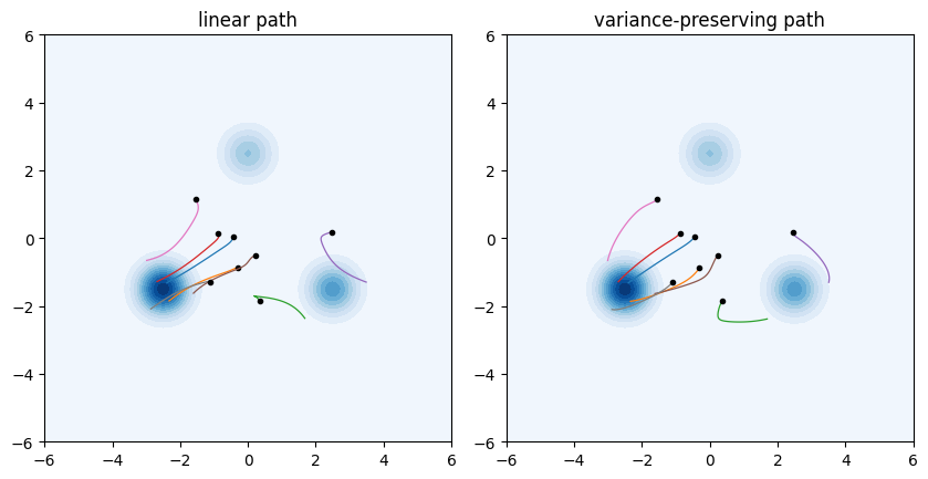
curvature of the exact flow, linear path: 0.213
curvature of the exact flow, variance-preserving path: 0.105
The exact flows of the linear and the variance-preserving path: both curved, the circle less so here. A straight conditional path does not make the marginal flow straight; reflow straightens it by changing the coupling.
The Same U-Net, a Velocity Target
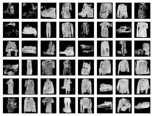
final training loss: 0.273Interpolate instead of noising, regress onto \mathbf{x}_1 - \mathbf{x}_0, integrate with fifty steps.
Recap
- Flow matching learns the velocity of a prescribed noise-to-data path; conditional flow matching makes it a regression on straight segments.
- For Gaussian paths, score and velocity are affine in the same posterior mean: diffusion is flow matching on the variance-preserving path.
- What differs: the path’s geometry, the target’s conditioning and weighting, the sampler.
- Next: the same ideas for discrete data.