Training Energy-Based Models

Dive into Deep Learning · §17.2

Training energy-based models
the gradient needs samples, not Z · Metropolis–Hastings · contrastive divergence and its cost

The Running Example: a Mixture with Known Density

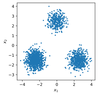
Three Gaussians in the plane, weights 0.5, 0.3, 0.2, standard deviation 0.5: closed-form density, closed-form score, and a reference test negative log-likelihood of about 2.5 nats.
key = jax.random.PRNGKey(0)
mix = GaussianMixture(means=[[-2.5, -1.5], [2.5, -1.5], [0.0, 2.5]],
                      weights=[0.5, 0.3, 0.2], std=0.5)
key, k1, k2 = jax.random.split(key, 3)
data, test = mix.sample(k1, 2000), mix.sample(k2, 2000)
print(f'test NLL under the true density: {-mix.log_prob(test).mean():.3f} nats')
d2l.set_figsize((3.5, 3.5))
d2l.plt.scatter(data[:, 0], data[:, 1], s=4)
d2l.plt.xlabel('$x_1$'), d2l.plt.ylabel('$x_2$');

test NLL under the true density: 2.474 nats

The Log-Partition Gradient Is a Model Expectation

\nabla_{\boldsymbol{\theta}} \log Z(\boldsymbol{\theta}) = -\,\mathbb{E}_{\mathbf{x} \sim p_{\boldsymbol{\theta}}}\big[\nabla_{\boldsymbol{\theta}} E_{\boldsymbol{\theta}}(\mathbf{x})\big]

\nabla_{\boldsymbol{\theta}} \tfrac{1}{n}\textstyle\sum_i \log p_{\boldsymbol{\theta}}(\mathbf{x}_i) = -\,\mathbb{E}_{\textrm{data}}\big[\nabla_{\boldsymbol{\theta}} E_{\boldsymbol{\theta}}\big] + \mathbb{E}_{p_{\boldsymbol{\theta}}}\big[\nabla_{\boldsymbol{\theta}} E_{\boldsymbol{\theta}}\big]

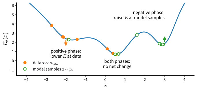
  • positive phase: lower the energy at data;
  • negative phase: raise it at model samples;
  • the update needs samples, not Z.

Two Phases on a One-Dimensional Energy

Where model samples coincide with data, the two pushes cancel and the energy stops changing.

The Identity, Checked Against Quadrature

In two dimensions the grid version of the model can be sampled exactly, so the two sides of the identity can be compared:

def flat_grad(fn, energy):
    return jax.flatten_util.ravel_pytree(nnx.grad(fn)(energy))[0]

grad_log_Z = flat_grad(log_Z, energy_mle)
probs = jax.nn.softmax(-energy_mle(grid), 0)  # p_theta on the grid
for n in (100, 1000, 10000):
    key, subkey = jax.random.split(key)
    x = grid[jax.random.choice(subkey, len(grid), (n,), p=probs)]  # x ~ p_theta
    grad_mc = flat_grad(lambda m: -m(x).mean(), energy_mle)  # -E_p[grad E]
    print(f'{n:>6d} model samples: relative error '
          f'{jnp.linalg.norm(grad_mc - grad_log_Z) / jnp.linalg.norm(grad_log_Z):.3f}')
   100 model samples: relative error 0.091
  1000 model samples: relative error 0.042
 10000 model samples: relative error 0.009

Monte Carlo error falls like 1/\sqrt{n}.

Metropolis–Hastings Uses Only Energy Differences

Propose \mathbf{x}' \sim Q(\cdot \mid \mathbf{x}), accept with

A = \min\left\{1,\ \frac{p_{\boldsymbol{\theta}}(\mathbf{x}')\, Q(\mathbf{x} \mid \mathbf{x}')}{p_{\boldsymbol{\theta}}(\mathbf{x})\, Q(\mathbf{x}' \mid \mathbf{x})}\right\} = \min\{1, e^{-\Delta E}\} \ \text{for a symmetric } Q.

  • Z cancels in the ratio;
  • detailed balance holds, so p_{\boldsymbol{\theta}} is stationary;
  • correctness is asymptotic; the mixing time decides the cost.

Step Size: Acceptance versus Mixing

def mode_weights(x):
    """The fraction of points closest to each component mean."""
    d2 = ((x[:, None, :] - mix.means[None]) ** 2).sum(-1)
    return [round(float(w), 3) for w in
            jnp.bincount(d2.argmin(1), length=3) / len(x)]

class TrueEnergy(nnx.Module):  # a parameter-free module, so it can be jitted
    def __call__(self, x):
        return -mix.log_prob(x)

true_energy = TrueEnergy()
key, subkey = jax.random.split(key)
x_init = 3 * jax.random.normal(subkey, (2000, 2))
print(f'true mode weights: {[round(w, 3) for w in mix.weights.tolist()]}')
for step_size in (0.25, 1.0, 4.0):
    key, subkey = jax.random.split(key)
    x, rate = metropolis_hastings(true_energy, x_init, subkey, 2000, step_size)
    d2 = ((x[:, None, :] - mix.means[None]) ** 2).sum(-1).min(1)
    print(f'step size {step_size}: acceptance {rate:.2f}, mode weights '
          f'{mode_weights(x)}, within-mode spread {d2.mean():.2f}')
true mode weights: [0.5, 0.3, 0.2]
step size 0.25: acceptance 0.76, mode weights [0.311, 0.334, 0.356], within-mode spread 0.51
step size 1.0: acceptance 0.29, mode weights [0.502, 0.295, 0.203], within-mode spread 0.52
step size 4.0: acceptance 0.06, mode weights [0.492, 0.299, 0.21], within-mode spread 0.49

Small steps: the within-mode spread is right, the weights are wrong. Large steps: the weights approach the truth, and most proposals are rejected.

Persistent Contrastive Divergence

Chains live across updates; twenty Metropolis–Hastings steps per gradient step keep them near the moving model.
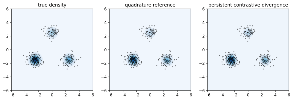
Within a few hundredths of a nat of the quadrature reference once the learning rate has decayed, at the cost of a sampling loop inside every update.

Recap

  • \nabla_{\boldsymbol{\theta}} \log Z = -\mathbb{E}_{p_{\boldsymbol{\theta}}}[\nabla_{\boldsymbol{\theta}} E]: maximum likelihood lowers the energy at data (positive phase) and raises it at model samples (negative phase).
  • Metropolis–Hastings samples from \exp(-E) with energy differences alone; its step size trades acceptance against mixing.
  • Contrastive divergence shortens the chains; the persistent variant reuses them. Both are biased by incomplete mixing.
  • The inner sampling loop is the cost. Next: an objective whose gradient needs no model samples.