From Fully Connected Layers to Convolutions
Fully connected layers do not scale
Distinguishing cats from dogs on one-megapixel photographs:
- Each input has 10^6 dimensions.
- Even an aggressive reduction to 1000 hidden units costs 10^6 \times 10^3 = 10^9 parameters for a single layer.
- Keep the hidden layer spatially organized at full resolution and the count reaches 10^{12}.
The objection is not that computers cannot hold 10^{12} numbers. It is waste: about a million times more parameters than the number of training images we could plausibly collect.
Images have structure we can exploit
Flattening an image into a vector forgets which pixels are neighbors. Yet humans and machines both classify pets easily, because natural images are far from arbitrary:
- Nearby pixels are strongly correlated.
- The same pattern (an edge, an eye, a whisker) means the same thing wherever it appears.
CNNs are one way of building this knowledge into the architecture itself.
Where’s Waldo?
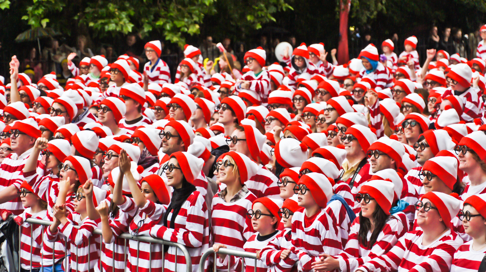
Can you find Waldo?
What Waldo looks like does not depend on where Waldo is located. So sweep the image with a Waldo detector: assign each patch a score for how likely it is to contain him. Many object detection and segmentation systems work this way.
Two principles
Desiderata for a vision architecture:
- Translation equivariance: in the earliest layers, shifting the input should shift the feature map by the same amount. The same patch gets the same response wherever it appears.
- Locality: early layers should look only at small neighborhoods, ignoring distant regions.
Deeper layers then aggregate: longer-range features first, image-level predictions at the end.
Constraining the MLP: the unconstrained case
Keep both input \mathbf{X} and hidden representation \mathbf{H} as 2-D grids. Fully connecting them takes a fourth-order weight tensor:
[\mathbf{H}]_{i, j} = [\mathbf{U}]_{i, j} + \sum_a \sum_b [\mathsf{V}]_{i, j, a, b} [\mathbf{X}]_{i+a, j+b}.
Every output location (i, j) owns its own full-image weight table. For a 1000 \times 1000 image: 10^{12} parameters.
Step 1: impose translation equivariance
A shift in \mathbf{X} should produce the same shift in \mathbf{H}. That forces the weights to be independent of location: [\mathsf{V}]_{i, j, a, b} = [\mathbf{V}]_{a, b}.
[\mathbf{H}]_{i, j} = u + \sum_a\sum_b [\mathbf{V}]_{a, b} [\mathbf{X}]_{i+a, j+b}.
One shared filter for the whole image: 10^{12} parameters become 4 \times 10^6.
Step 2: impose locality
Outside a small window, set the weights to zero: [\mathbf{V}]_{a, b} = 0 for |a| > \Delta or |b| > \Delta.
[\mathbf{H}]_{i, j} = u + \sum_{a = -\Delta}^{\Delta} \sum_{b = -\Delta}^{\Delta} [\mathbf{V}]_{a, b} [\mathbf{X}]_{i+a, j+b}.
With \Delta < 10, the count drops from roughly 4 \times 10^6 to (2\Delta+1)^2: a few hundred parameters.
This is a convolutional layer, and \mathbf{V} is its kernel (or filter).
Why is it called a convolution?
In mathematics, the convolution of two functions is
(f * g)(i, j) = \sum_a\sum_b f(a, b) g(i-a, j-b).
Our layer uses (i+a, j+b) instead of (i-a, j-b): strictly speaking it computes a cross-correlation. The difference is cosmetic (flip the kernel), and deep learning keeps the name convolution.
Equivariance vs. invariance
Let T_v translate an image by offset v. For a map f:
\begin{aligned} f(T_v \mathbf{X}) &= T_v f(\mathbf{X}) && \text{(equivariance)},\\ f(T_v \mathbf{X}) &= f(\mathbf{X}) && \text{(invariance)}.\end{aligned}
- Convolutional layers are equivariant: shift the input, the feature map shifts along.
- Invariance is supplied by the head of the network: pooling and aggregation discard where a feature occurred and keep only whether it occurred.
Channels
Images are not 2-D: an RGB input is a third-order tensor, e.g., 1024 \times 1024 \times 3. Hidden representations become stacks of 2-D grids too, called channels or feature maps:
[\mathsf{H}]_{i,j,d} = \sum_{a = -\Delta}^{\Delta} \sum_{b = -\Delta}^{\Delta} \sum_c [\mathsf{V}]_{a, b, c, d} [\mathsf{X}]_{i+a, j+b, c}.
The kernel gains two channel indices: c sums over input channels, d selects the output channel. Different channels can specialize, e.g., to edges or textures.
A Waldo detector, concretely
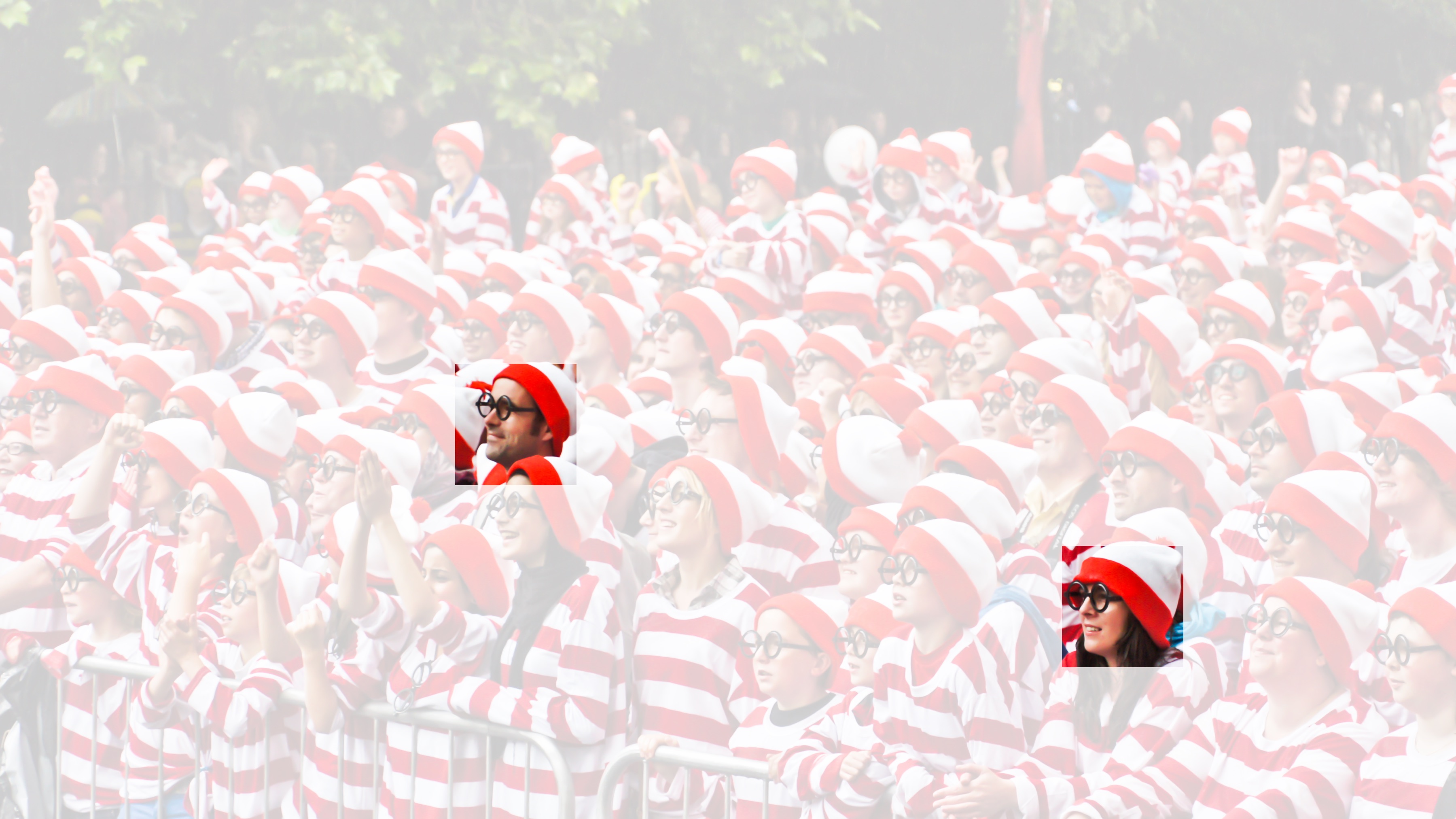
The filter response peaks at Waldo’s location.
Slide the learned filter \mathsf{V} over the image and weigh intensities window by window; wherever the “waldoness” is highest, the hidden representation should peak.
What remains: combining feature maps into a single answer (is Waldo anywhere?), efficient computation, and stacking layers. That is the rest of this chapter.
Recap
- Flattening images into vectors discards spatial structure and wastes parameters.
- Two principles constrain the MLP: translation equivariance (share weights across locations) and locality (small windows).
- Applying both turns a 10^{12}-parameter layer into a convolutional layer with a few hundred parameters.
- Convolutional layers are translation equivariant; the network head buys invariance by aggregation.
- Channels restore expressive power: many filters per layer, operating over all input channels.