Wrapping as a Module

Batch Normalization

BatchNorm stabilizes deep nets

Batch Normalization (Ioffe & Szegedy, 2015) is the single-biggest stability win in modern deep learning.

At each layer, normalize activations within the minibatch to zero mean / unit variance, then rescale with learned \gamma and \beta:

\text{BN}(\mathbf{x}) = \gamma \cdot \frac{\mathbf{x} - \hat\mu_\mathcal{B}}{\sqrt{\hat\sigma_\mathcal{B}^2 + \epsilon}} + \beta.

Why it works

• Lets you train much deeper nets — gradients stay well-conditioned through the depth.
• Allows higher learning rates; mildly regularizing.
• Test time uses running estimates of mean / variance (no minibatch then).
• Spawned a family — LayerNorm (per-example, used in Transformers), GroupNorm, InstanceNorm.

From scratch

Compute per-channel mean and variance over the minibatch (and spatial dims, for conv); normalize, then scale + shift:

from d2l import jax as d2l
from flax import linen as nn
from functools import partial
from jax import numpy as jnp
import jax
import optax

def batch_norm(X, deterministic, gamma, beta, moving_mean, moving_var, eps,
               momentum):
    # Use `deterministic` to determine whether the current mode is training
    # mode or prediction mode
    if deterministic:
        # In prediction mode, use mean and variance obtained by moving average
        # `linen.Module.variables` have a `value` attribute containing the array
        X_hat = (X - moving_mean.value) / jnp.sqrt(moving_var.value + eps)
    else:
        assert len(X.shape) in (2, 4)
        if len(X.shape) == 2:
            # When using a fully connected layer, calculate the mean and
            # variance on the feature dimension
            mean = X.mean(axis=0)
            var = ((X - mean) ** 2).mean(axis=0)
        else:
            # When using a two-dimensional convolutional layer, calculate the
            # mean and variance on the channel dimension (axis=1). Here we
            # need to maintain the shape of `X`, so that the broadcasting
            # operation can be carried out later
            mean = X.mean(axis=(0, 2, 3), keepdims=True)
            var = ((X - mean) ** 2).mean(axis=(0, 2, 3), keepdims=True)
        # In training mode, the current mean and variance are used
        X_hat = (X - mean) / jnp.sqrt(var + eps)
        # Update the mean and variance using moving average
        moving_mean.value = momentum * moving_mean.value + (1.0 - momentum) * mean
        moving_var.value = momentum * moving_var.value + (1.0 - momentum) * var
    Y = gamma * X_hat + beta  # Scale and shift
    return Y

Buffers for moving_mean / moving_var (updated only during training); learnable gamma / beta parameters:

class BatchNorm(nn.Module):
    # `num_features`: the number of outputs for a fully connected layer
    # or the number of output channels for a convolutional layer.
    # `num_dims`: 2 for a fully connected layer and 4 for a convolutional layer
    # Use `deterministic` to determine whether the current mode is training
    # mode or prediction mode
    num_features: int
    num_dims: int
    deterministic: bool = False

    @nn.compact
    def __call__(self, X):
        if self.num_dims == 2:
            shape = (1, self.num_features)
        else:
            shape = (1, 1, 1, self.num_features)

        # The scale parameter and the shift parameter (model parameters) are
        # initialized to 1 and 0, respectively
        gamma = self.param('gamma', jax.nn.initializers.ones, shape)
        beta = self.param('beta', jax.nn.initializers.zeros, shape)

        # The variables that are not model parameters are initialized to 0 and
        # 1. Save them to the 'batch_stats' collection
        moving_mean = self.variable('batch_stats', 'moving_mean', jnp.zeros, shape)
        moving_var = self.variable('batch_stats', 'moving_var', jnp.ones, shape)
        Y = batch_norm(X, self.deterministic, gamma, beta,
                       moving_mean, moving_var, eps=1e-5, momentum=0.9)

        return Y

LeNet + BatchNorm

Drop a BatchNorm layer between each conv/linear and its activation:

class BNLeNetScratch(d2l.Classifier):
    lr: float = 0.1
    num_classes: int = 10
    training: bool = True

    def setup(self):
        self.net = nn.Sequential([
            nn.Conv(6, kernel_size=(5, 5)),
            BatchNorm(6, num_dims=4, deterministic=not self.training),
            nn.sigmoid,
            lambda x: nn.avg_pool(x, window_shape=(2, 2), strides=(2, 2)),
            nn.Conv(16, kernel_size=(5, 5)),
            BatchNorm(16, num_dims=4, deterministic=not self.training),
            nn.sigmoid,
            lambda x: nn.avg_pool(x, window_shape=(2, 2), strides=(2, 2)),
            lambda x: x.reshape((x.shape[0], -1)),
            nn.Dense(120),
            BatchNorm(120, num_dims=2, deterministic=not self.training),
            nn.sigmoid,
            nn.Dense(84),
            BatchNorm(84, num_dims=2, deterministic=not self.training),
            nn.sigmoid,
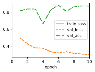
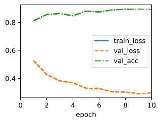
            nn.Dense(self.num_classes)])

Train

Trains noticeably faster than vanilla LeNet — same accuracy in fewer epochs:

trainer = d2l.Trainer(max_epochs=10, num_gpus=1)
data = d2l.FashionMNIST(batch_size=128)
model = BNLeNetScratch(lr=0.1)
trainer.fit(model, data)

After training, gamma and beta are non-trivial — the layer learned the scale/shift it wants:

trainer.state.params['net']['layers_1']['gamma'].reshape((-1,)), \
trainer.state.params['net']['layers_1']['beta'].reshape((-1,))

(Array([2.2793572, 2.1558688, 1.6549996, 1.3313813, 1.8517964, 2.6196404],      dtype=float32),
 Array([-0.38942158, -0.4962455 ,  0.0702681 , -0.26407185,  0.3260278 ,
         0.7118782 ], dtype=float32))

The framework version

nn.BatchNorm2d for conv layers, nn.BatchNorm1d for linear layers — same idea, much faster, handles the eval/training mode switch automatically:

class BNLeNet(d2l.Classifier):
    lr: float = 0.1
    num_classes: int = 10
    training: bool = True

    def setup(self):
        # Flax's default momentum=0.99 decays the OLD running stats; PT/MX use
        # momentum=0.1 on the NEW stats, i.e. decay-of-OLD = 0.9. Pass 0.9 to
        # match the other tabs.
        self.net = nn.Sequential([
            nn.Conv(6, kernel_size=(5, 5)),
            nn.BatchNorm(not self.training, momentum=0.9),
            nn.sigmoid,
            lambda x: nn.avg_pool(x, window_shape=(2, 2), strides=(2, 2)),
            nn.Conv(16, kernel_size=(5, 5)),
            nn.BatchNorm(not self.training, momentum=0.9),
            nn.sigmoid,
            lambda x: nn.avg_pool(x, window_shape=(2, 2), strides=(2, 2)),
            lambda x: x.reshape((x.shape[0], -1)),
            nn.Dense(120),
            nn.BatchNorm(not self.training, momentum=0.9),
            nn.sigmoid,
            nn.Dense(84),
            nn.BatchNorm(not self.training, momentum=0.9),
            nn.sigmoid,
            nn.Dense(self.num_classes)])

trainer = d2l.Trainer(max_epochs=10, num_gpus=1)
data = d2l.FashionMNIST(batch_size=128)
model = BNLeNet(lr=0.1)
trainer.fit(model, data)

Recap

• BatchNorm normalizes activations to zero mean / unit variance within each minibatch, then rescales with learned \gamma, \beta.
• Track running statistics during training; use them at inference (no minibatch at test time).
• Enables much deeper networks, higher LRs, faster convergence; mildly regularizing.
• Spawned a family — LayerNorm (per-example, used in Transformers), GroupNorm, InstanceNorm.