Shape inspection

Deep Convolutional Neural Networks (AlexNet)

AlexNet: scale changes vision

AlexNet (Krizhevsky, Sutskever, Hinton — 2012) is what made deep learning the approach to vision. Won ImageNet by a huge margin and started the modern era.

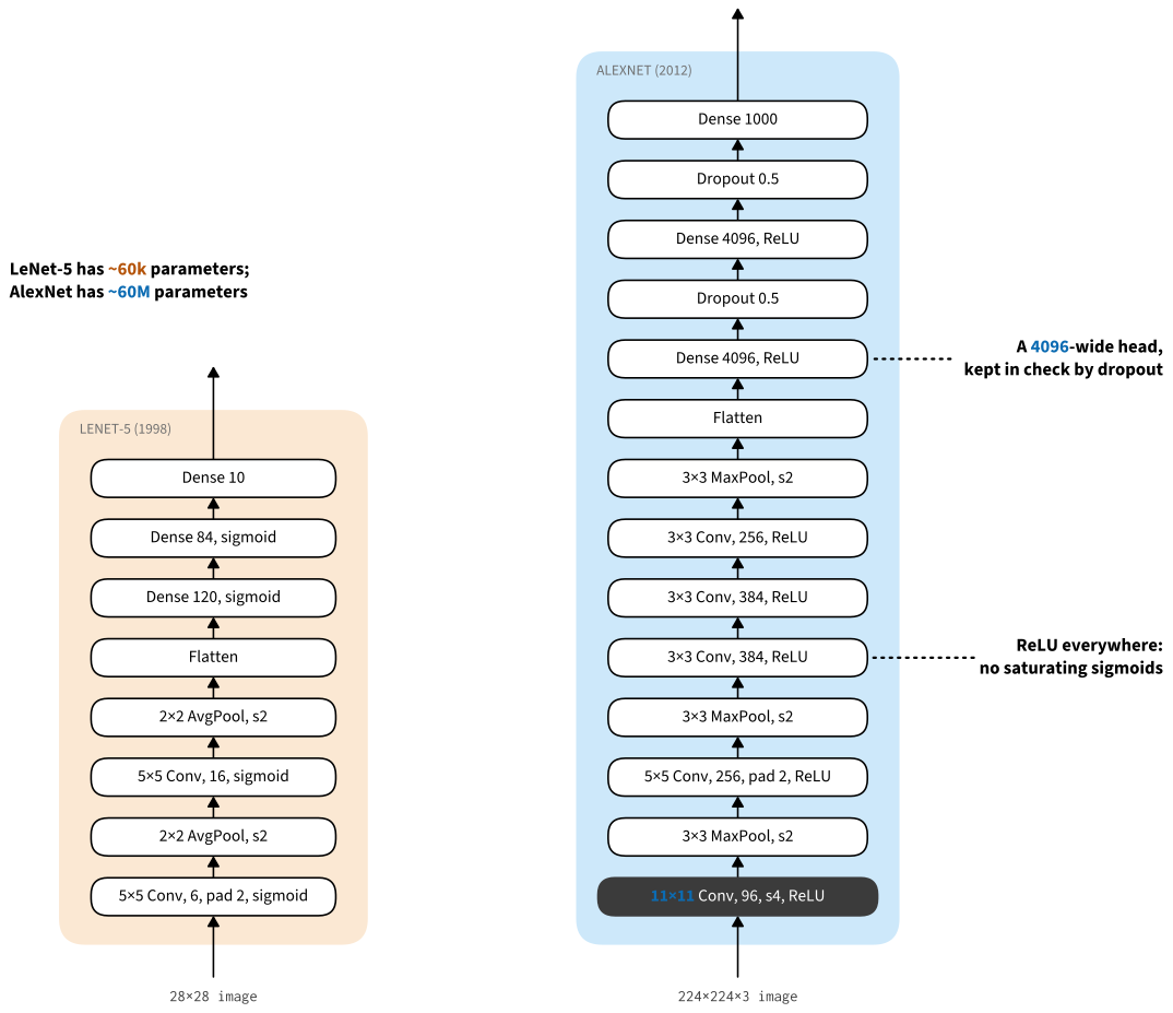
AlexNet alongside the LeNet from a decade earlier.

What changed from LeNet

• Bigger — 8 layers, 60 M parameters, larger first-layer filters (11×11), deeper feature stack.
• ReLU activations (no more saturating sigmoids).
• Dropout in the dense head for regularization.
• GPUs, ImageNet (1.2 M images), and augmentation — the missing ingredients.

The architecture itself is straightforward; what changed was the scale.

The architecture in code

Five conv layers (11×11 → 5×5 → three 3×3) + max-pool, then three FC layers down to 1000 classes:

from d2l import jax as d2l
from flax import linen as nn
import jax
from jax import numpy as jnp

class AlexNet(d2l.Classifier):
    lr: float = 0.1
    num_classes: int = 10
    training: bool = True

    def setup(self):
        self.net = nn.Sequential([
            nn.Conv(features=96, kernel_size=(11, 11), strides=4, padding=1),
            nn.relu,
            lambda x: nn.max_pool(x, window_shape=(3, 3), strides=(2, 2)),
            nn.Conv(features=256, kernel_size=(5, 5)),
            nn.relu,
            lambda x: nn.max_pool(x, window_shape=(3, 3), strides=(2, 2)),
            nn.Conv(features=384, kernel_size=(3, 3)), nn.relu,
            nn.Conv(features=384, kernel_size=(3, 3)), nn.relu,
            nn.Conv(features=256, kernel_size=(3, 3)), nn.relu,
            lambda x: nn.max_pool(x, window_shape=(3, 3), strides=(2, 2)),
            lambda x: x.reshape((x.shape[0], -1)),  # flatten
            nn.Dense(features=4096),
            nn.relu,
            nn.Dropout(0.5, deterministic=not self.training),
            nn.Dense(features=4096),
            nn.relu,
            nn.Dropout(0.5, deterministic=not self.training),
            nn.Dense(features=self.num_classes)
        ])

Walk a single 1×1×224×224 image through and print each block’s output shape — the feature pyramid going from 224×224×1 down to 6×6×256:

AlexNet(training=False).layer_summary((1, 224, 224, 1))

Conv output shape:   (1, 54, 54, 96)
custom_jvp output shape:     (1, 54, 54, 96)
function output shape:   (1, 26, 26, 96)
Conv output shape:   (1, 26, 26, 256)
custom_jvp output shape:     (1, 26, 26, 256)
function output shape:   (1, 12, 12, 256)
...
custom_jvp output shape:     (1, 4096)
Dropout output shape:    (1, 4096)
Dense output shape:  (1, 4096)
custom_jvp output shape:     (1, 4096)
Dropout output shape:    (1, 4096)
Dense output shape:  (1, 10)

Training on Fashion-MNIST

For demonstration, upsample the 28×28 Fashion-MNIST images to the 224×224 input AlexNet expects, then train at lr=0.01:

model = AlexNet(lr=0.01)
data = d2l.FashionMNIST(batch_size=128, resize=(224, 224))
trainer = d2l.Trainer(max_epochs=10, num_gpus=1)
trainer.fit(model, data)

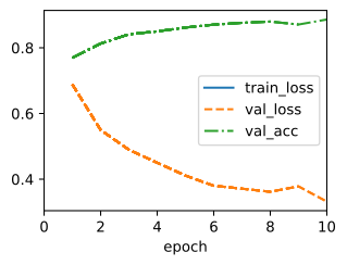
Trains slowly even on a GPU — AlexNet has ~10× the parameters of LeNet. The architecture’s lasting contribution: it proved that bigger is better when paired with enough data and compute.

Recap

• AlexNet = LeNet’s recipe at 8× the depth, massive parameter count, ReLU, Dropout, GPU training, on ImageNet.
• Validates the “deeper, bigger, more data” formula that drives the field for the next decade.
• The next handful of architectures (VGG, GoogLeNet, ResNet) are systematic refinements of this template.