Fine-Tuning

You’ll rarely train a vision model from scratch. Transfer learning — start from weights pretrained on a big dataset (ImageNet) and adapt to your small one — is the default recipe.

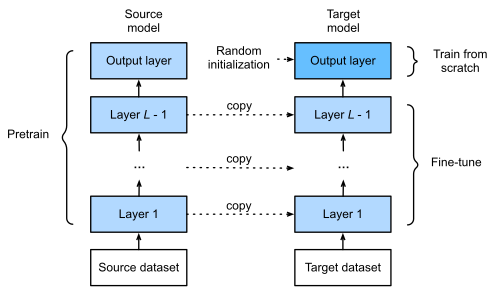
Fine-tuning: pretrained backbone + new task-specific head.

The standard recipe

Take a pretrained network (ResNet, ViT, etc.).
Replace the output layer with a head for your task.
Optionally freeze early layers; train the rest.
Small LR on the pretrained part, larger LR on the new head.

Setup

%matplotlib inline
import os
from d2l import jax as d2l
from d2l.nnx_resnet import ResNet50, Bottleneck
from flax import nnx
import jax
from jax import numpy as jnp
import optax
import numpy as np
import tensorflow as tf  # only used for tf.data input pipeline

# Activation (gradient) checkpointing. Fine-tuning ResNet-50 at batch size 128
# would otherwise hold the whole forward graph's activations live for the
# backward pass (~23 GB). Wrapping each residual block (`Bottleneck`) in
# `nnx.remat` recomputes that block's activations during backprop instead of
# storing them, cutting the peak to ~6 GB. `nnx.remat` propagates state
# correctly, so gradients and batch-norm running statistics are identical to
# the un-checkpointed model.
if not getattr(Bottleneck, '_d2l_remat', False):
    Bottleneck.__call__ = nnx.remat(Bottleneck.__call__)
    Bottleneck._d2l_remat = True

The hot-dog dataset

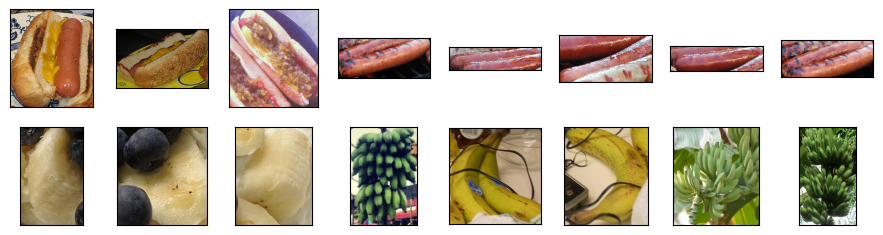
A tiny binary classification dataset (hot dog / not hot dog) — too small to train a CNN from scratch, perfect for transfer learning:

d2l.DATA_HUB['hotdog'] = (d2l.DATA_URL + 'hotdog.zip', 
                         'fba480ffa8aa7e0febbb511d181409f899b9baa5')

data_dir = d2l.download_extract('hotdog')

# Load images as (PIL.Image, label) lists for compatibility with show_images
from PIL import Image as _PILImage
import pathlib

def _load_image_folder(path):
    """Load images from a directory with class subfolders, returning
    a list of (PIL.Image, class_index) tuples."""
    path = pathlib.Path(path)
    class_names = sorted([p.name for p in path.iterdir() if p.is_dir()])
    class_to_idx = {c: i for i, c in enumerate(class_names)}
    items = []
    for cls in class_names:
        for img_path in sorted((path / cls).iterdir()):
            try:
                img = _PILImage.open(str(img_path)).convert('RGB')
                items.append((img, class_to_idx[cls]))
            except Exception:
                continue
    return items

train_imgs = _load_image_folder(os.path.join(data_dir, 'train'))
test_imgs = _load_image_folder(os.path.join(data_dir, 'test'))

hotdogs = [train_imgs[i][0] for i in range(8)]
not_hotdogs = [train_imgs[-i - 1][0] for i in range(8)]
d2l.show_images(hotdogs + not_hotdogs, 2, 8, scale=1.4);

Augmentation pipelines

Standard ImageNet recipe — random resized crop + flip for training, center crop for eval. Match the preprocessing convention that the pretrained model expects:

# Image preprocessing. We use `tf.image` ops so the pipeline can run
# inside `tf.data.Dataset.map`. The ImageNet RGB mean/std normalization
# matches the preprocessing expected by the pretrained ImageNet ResNet
# weights (and the PyTorch/MXNet tabs).
IMG_SIZE = 224
_IMAGENET_MEAN = tf.constant([0.485, 0.456, 0.406], dtype=tf.float32)
_IMAGENET_STD  = tf.constant([0.229, 0.224, 0.225], dtype=tf.float32)

def _normalize(x):
    return (tf.cast(x, tf.float32) / 255.0 - _IMAGENET_MEAN) / _IMAGENET_STD

def train_preprocess(x):
    # `x` is a (256, 256, 3) float32 RGB image with values in [0, 255].
    x = tf.image.random_crop(x, size=(IMG_SIZE, IMG_SIZE, 3))
    x = tf.image.random_flip_left_right(x)
    return _normalize(x)

def test_preprocess(x):
    x = tf.image.resize_with_crop_or_pad(x, IMG_SIZE, IMG_SIZE)
    return _normalize(x)

Inspect the pretrained head

The source model was trained for 1000 ImageNet classes. Its convolutional body is reusable; the final classifier is task-specific and will be replaced:

_dummy = jnp.zeros((1, IMG_SIZE, IMG_SIZE, 3), dtype=jnp.float32)
pretrained_net = ResNet50.from_pretrained()

Downloading bytes:           |  0.00B            
Reconstructing (incomplete total...): |          |  0.00B /  0.00B            
Fetching 1 files:   0%|          | 0/1 [00:00<?, ?it/s]

Replace the task head

Create a target model with the same pretrained backbone and a randomly initialized 2-way classifier for hot dog vs. not hot dog:

pretrained_net.fc.kernel.shape

(2048, 1000)

Discriminative learning rates

Let \theta_b be pretrained backbone parameters and \theta_h the new head. Use a small step on \theta_b and a larger one on \theta_h:

\eta_b = \eta,\qquad \eta_h = 10\eta.

finetune_net = ResNet50.from_pretrained()
finetune_net.fc = nnx.Linear(2048, 2, rngs=nnx.Rngs(1))

Downloading bytes:           |  0.00B            
Reconstructing (incomplete total...): |          |  0.00B /  0.00B            
Fetching 1 files:   0%|          | 0/1 [00:00<?, ?it/s]

Training helper

The helper hides framework details: parameter groups, optimizer construction, metric logging, and the scratch/fine-tune switch. The four-step pattern is:

build the pretrained backbone and new head;
assign a small learning rate to backbone parameters;
assign a larger learning rate to the randomly initialized head;
train and compare against a scratch baseline.

Run fine-tuning

With matched ImageNet preprocessing and a small base LR, the pretrained model should reach useful accuracy quickly. The point is not just a better final score; it is much less data and compute than training the same network cold.

print('fine-tuned model')
finetune_net = train_fine_tuning(finetune_net, 1e-4, momentum=0.9)

fine-tuned model
E0719 14:24:38.739296 46176 cuda_timer.cc:88] Delay kernel timed out: measured time has sub-optimal accuracy. There may be a missing warmup execution, ...
epoch 1, loss 0.637, train acc 0.780, test acc 0.873
epoch 2, loss 0.524, train acc 0.906, test acc 0.911
epoch 3, loss 0.420, train acc 0.934, test acc 0.917
epoch 4, loss 0.342, train acc 0.942, test acc 0.921
epoch 5, loss 0.284, train acc 0.944, test acc 0.926

From-scratch baseline

Same architecture, no pretraining. Much worse on this small dataset — illustrates why transfer learning is the default:

print('scratch baseline')
scratch_net = ResNet50(num_classes=2, rngs=nnx.Rngs(2))
# On this tiny dataset the running statistics must adapt much faster than the
# ImageNet default.
scratch_net = nnx.view(scratch_net, momentum=0.5, raise_if_not_found=False)
scratch_net = train_fine_tuning(
    scratch_net, 1e-3, num_epochs=6, param_group=False,
    update_batch_stats=True, momentum=0.9)

scratch baseline
epoch 1, loss 0.689, train acc 0.545, test acc 0.564
epoch 2, loss 0.651, train acc 0.620, test acc 0.497
epoch 3, loss 0.630, train acc 0.654, test acc 0.559
epoch 4, loss 0.494, train acc 0.779, test acc 0.566
epoch 5, loss 0.367, train acc 0.838, test acc 0.655
epoch 6, loss 0.352, train acc 0.845, test acc 0.771

What to vary

The natural ablations are: freeze more or fewer layers, change the backbone/head learning-rate ratio, and compare against the source ImageNet “hotdog” class weights.

# Freeze the pretrained ResNet-50 backbone; only the new `fc` head
# is updated by setting the optimizer learning rate of every other parameter
# to zero. For example, modify `train_fine_tuning` to use:
#   optax.multi_transform(
#       {'head': optax.sgd(lr * 10, momentum=0.9),
#        'base': optax.set_to_zero()},
#       labels)

# The pretrained classifier maps 2048-dimensional features to 1000 classes.
weight = pretrained_net.fc.kernel[...]  # Shape: (2048, 1000)
hotdog_w = weight[:, 934]
hotdog_w.shape

(2048,)

Recap

Transfer learning: pretrained backbone + new head; almost always beats from-scratch on small / medium datasets.
Use small LR on the backbone (10×–100× smaller than the head LR) — pretrained features need only nudges.
Match input preprocessing (mean/std normalization, input size, or model-specific preprocess_input) to what the pretrained model expects.
Modern variants: feature-extractor mode (freeze everything but head), full fine-tune (everything trains), parameter-efficient methods (LoRA, adapters).