device = jax.devices()[0]
peak_tflops = 165.0   # RTX 4090 dense bf16 tensor-core spec
bandwidth_tbs = 1.008  # GDDR6X spec
print(f'{device.device_kind}')
print(f'ridge point = {peak_tflops / bandwidth_tbs:.0f} FLOP/byte')Arithmetic Intensity and the Roofline
Every op asks for FLOPs and bytes. Intensity = FLOPs/byte.
\textrm{performance} \leq \min(P,\; I \cdot \beta)
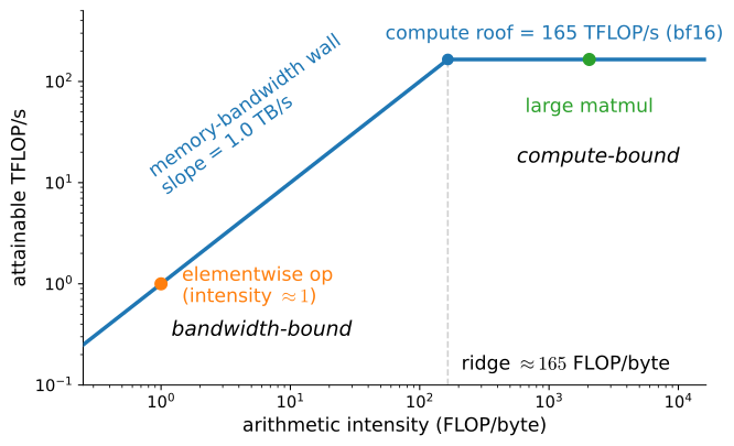
Matmul \mathbf{X}_{B\times D}\mathbf{W}_{D\times F}: intensity \approx 2B/b — batch size is intensity. Elementwise ops: intensity below 1, forever bandwidth-bound.
Correct GPU Timing
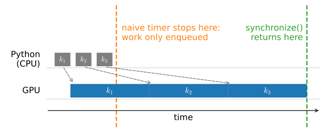
Dispatch is asynchronous — Python enqueues, the GPU runs behind.
key = jax.random.PRNGKey(0)
a = jax.random.normal(key, (4096, 4096), dtype=jnp.bfloat16)
jnp.dot(a, a).block_until_ready()  # Warmup: triggers compilation

t0 = time.perf_counter()
for _ in range(10):
    b = jnp.dot(a, a)
naive = time.perf_counter() - t0

b.block_until_ready()  # Drain the naive loop's in-flight work first
t0 = time.perf_counter()
for _ in range(10):
    b = jnp.dot(a, a)
b.block_until_ready()
honest = time.perf_counter() - t0
print(f'naive timer: {1000 * naive:.2f} ms   '
      f'with block_until_ready: {1000 * honest:.2f} ms')
naive timer: 0.74 ms with block_until_ready: 8.84 msOne Kernel across Three Regimes
sizes = [256, 512, 1024, 2048, 4096, 8192]
achieved = []
for n in sizes:
    a = jax.random.normal(key, (n, n), dtype=jnp.bfloat16)
    compiled = jax.jit(jnp.dot).lower(a, a).compile()
    flops = compiled.cost_analysis()['flops']  # Analytic count, no timing
    t = Benchmark(lambda: compiled(a, a)).time
    achieved.append(flops / t / 1e12)
d2l.plot(sizes, [achieved], 'matrix size $n$', 'achieved TFLOP/s',
         xscale='log', yscale='log')
print([f'{n}: {tf:.1f}' for n, tf in zip(sizes, achieved)])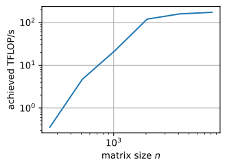
['256: 0.4', '512: 4.7', '1024: 21.8', '2048: 119.9', '4096: 158.7', '8192: 173.1']Small matrices are overhead-bound because launch time rivals arithmetic. Intermediate matrices use an increasing fraction of the 128 SMs. Large matrices approach the compute roof. The roofline is the ceiling; the measured knee (~2048–4096) sits well past the nominal crossover (~500) — that gap is utilization and overhead.
Diagnosis Determines the Fix
x = jax.random.normal(key, (4000, 4000))
for desc, f in [('add', lambda: x + 1), ('mul', lambda: x * 1.5),
                ('sin', lambda: jnp.sin(x)),
                ('sigmoid', lambda: jax.nn.sigmoid(x))]:
    print(Benchmark(f, desc=desc))
add: 0.29 ms/call
mul: 0.30 ms/call
sin: 0.17 ms/call
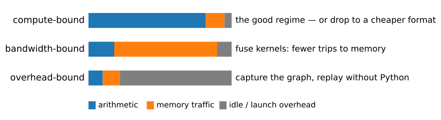
sigmoid: 0.16 ms/callBelow the ridge, sin and addition take similar time because memory traffic, rather than arithmetic, determines elapsed time.