Toy network

Training on Multiple GPUs

Scaling beyond one GPU

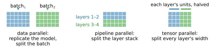
A single GPU can train ResNet on ImageNet — slowly. Modern large models need many GPUs. Three ways to split work:

• Network partitioning — different layers on different GPUs. Hard to balance; rarely used alone today.
• Layerwise partitioning — split each layer’s parameters across GPUs (model parallelism). For giant models whose weights don’t fit on one GPU.
• Data parallelism — replicate the model on every GPU; each processes a different minibatch chunk; gradients averaged across GPUs.

Data parallelism is the default for everyday training.

Strategies side by side

Original, network partitioning, layerwise partitioning, data parallelism.

Data parallelism

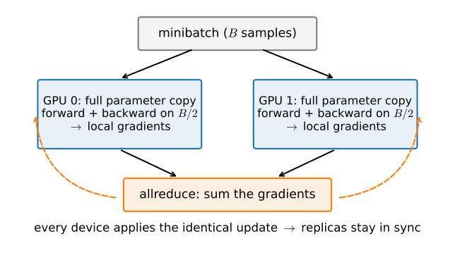
Each GPU computes a forward + backward pass on its slice of the minibatch. After the backward pass, gradients are averaged across GPUs (all_reduce). Optimizer step then runs identically on every GPU, keeping replicas in sync.

Data-parallel SGD on 2 GPUs: split data, compute gradients independently, all-reduce, then update.

%matplotlib inline
from d2l import jax as d2l
import jax
from jax import numpy as jnp
import numpy as np

Tiny LeNet for the demo — small enough to fit on each GPU many times over:

import functools
import optax

# Initialize model parameters
scale = 0.01
key = jax.random.PRNGKey(0)
keys = jax.random.split(key, 4)
W1 = jax.random.normal(keys[0], (20, 1, 3, 3)) * scale
b1 = jnp.zeros(20)
W2 = jax.random.normal(keys[1], (50, 20, 5, 5)) * scale
b2 = jnp.zeros(50)
W3 = jax.random.normal(keys[2], (800, 128)) * scale
b3 = jnp.zeros(128)
W4 = jax.random.normal(keys[3], (128, 10)) * scale
b4 = jnp.zeros(10)
params = [W1, b1, W2, b2, W3, b3, W4, b4]

# Define the model
def lenet(params, X):
    h1_conv = jax.lax.conv_general_dilated(
        X, params[0], window_strides=(1, 1), padding='VALID',
        dimension_numbers=('NCHW', 'OIHW', 'NCHW'))
    h1_conv = h1_conv + params[1].reshape(1, -1, 1, 1)
    h1_activation = jax.nn.relu(h1_conv)
    # Average pooling
    h1 = jax.lax.reduce_window(
        h1_activation, 0.0, jax.lax.add, (1, 1, 2, 2), (1, 1, 2, 2),
        'VALID') / 4.0
    h2_conv = jax.lax.conv_general_dilated(
        h1, params[2], window_strides=(1, 1), padding='VALID',
        dimension_numbers=('NCHW', 'OIHW', 'NCHW'))
    h2_conv = h2_conv + params[3].reshape(1, -1, 1, 1)
    h2_activation = jax.nn.relu(h2_conv)
    h2 = jax.lax.reduce_window(
        h2_activation, 0.0, jax.lax.add, (1, 1, 2, 2), (1, 1, 2, 2),
        'VALID') / 4.0
    h2 = h2.reshape(h2.shape[0], -1)
    h3_linear = jnp.dot(h2, params[4]) + params[5]
    h3 = jax.nn.relu(h3_linear)
    y_hat = jnp.dot(h3, params[6]) + params[7]
    return y_hat

Distribute parameters

Replicate the parameter list onto each device:

def get_params(params, num_devices):
    """Replicate parameters across multiple devices."""
    return jax.tree.map(
        lambda x: jnp.stack([x] * num_devices), params)

replicated = get_params(params, 1)
print('b1 weight:', replicated[1])
print('b1 devices:', replicated[1].devices())

b1 weight: [[0. 0. 0. 0. 0. 0. 0. 0. 0. 0. 0. 0. 0. 0. 0. 0. 0. 0. 0. 0.]]
b1 devices: {CudaDevice(id=0)}

all_reduce

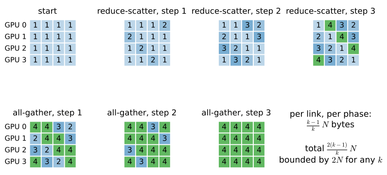
Sum vectors across GPUs and broadcast the result back — the gradient-averaging primitive of data-parallel SGD. NCCL implements this efficiently in production:

# In JAX, allreduce is done inside pmap via jax.lax.psum/pmean.
# Here we demonstrate with a simple pmap example.
devices = jax.local_devices()[:2]
data = jnp.stack([jnp.ones((1, 2)) * (i + 1) for i in range(2)])
print('before allreduce:\n', data[0], '\n', data[1])
summed = jax.pmap(lambda x: jax.lax.psum(x, axis_name='i'),
                  axis_name='i')(data)
print('after allreduce:\n', summed[0], '\n', summed[1])

before allreduce:
 [[1. 1.]] 
 [[2. 2.]]
after allreduce:
 [[3. 3.]] 
 [[3. 3.]]

Distribute the minibatch

Split a tensor evenly across devices:

data = jnp.arange(20).reshape(4, 5)
devices = jax.local_devices()[:2]
mesh = jax.sharding.Mesh(np.array(devices), ('dev',))
sharding = jax.sharding.NamedSharding(mesh, jax.sharding.PartitionSpec('dev'))
split = jax.device_put(data.reshape(2, 2, 5), sharding)
print('input :', data)
print('load into', devices)
print('output:', split)

input : [[ 0  1  2  3  4]
 [ 5  6  7  8  9]
 [10 11 12 13 14]
 [15 16 17 18 19]]
load into [CudaDevice(id=0), CudaDevice(id=1)]
output: 
[[[ 0  1  2  3  4]
  [ 5  6  7  8  9]]

 [[10 11 12 13 14]
  [15 16 17 18 19]]]

def split_batch(X, y, num_devices):
    """Split `X` and `y` across devices by reshaping."""
    assert X.shape[0] == y.shape[0]
    batch_size = X.shape[0]
    # Reshape (batch, ...) -> (num_devices, batch_per_device, ...)
    def _reshape(a):
        return a.reshape(num_devices, batch_size // num_devices, *a.shape[1:])
    return _reshape(X), _reshape(y)

One step of multi-GPU training

Forward + backward on each replica → all_reduce gradients → update parameters identically:

@functools.partial(jax.pmap, axis_name='batch',
                   static_broadcasted_argnums=(3,))
def pmap_step(params, X_shard, y_shard, lr):
    """One training step executed in parallel on each device."""
    def loss_fn(p):
        y_hat = lenet(p, X_shard)
        return jnp.mean(optax.softmax_cross_entropy_with_integer_labels(
            y_hat, y_shard))
    grads = jax.grad(loss_fn)(params)
    # All-reduce: sum gradients across devices
    grads = jax.lax.pmean(grads, axis_name='batch')
    # SGD update
    params = jax.tree.map(lambda p, g: p - lr * g, params, grads)
    return params

def train_batch(replicated_params, X, y, num_gpus, lr):
    X_shards, y_shards = split_batch(X, y, num_gpus)
    replicated_params = pmap_step(
        replicated_params, X_shards, y_shards, lr)
    return replicated_params

def evaluate_accuracy_jax(predict_fn, data_iter):
    """Evaluate accuracy using JAX predict function."""
    num_correct, num_total = 0, 0
    for X, y in data_iter:
        X, y = jnp.array(X).transpose(0, 3, 1, 2), jnp.array(y)
        y_hat = predict_fn(X)
        num_correct += jnp.sum(jnp.argmax(y_hat, axis=1) == y).item()
        num_total += y.shape[0]
    return num_correct / num_total

def train(num_gpus, batch_size, lr):
    data = d2l.FashionMNIST(batch_size=batch_size)
    train_iter = data.get_dataloader(train=True)
    test_iter = data.get_dataloader(train=False)
    devices = jax.local_devices()[:num_gpus]
    # Replicate model parameters to `num_gpus` GPUs
    replicated_params = jax.tree.map(
        lambda x: jnp.stack([x] * num_gpus), params)
    num_epochs = 10
    animator = d2l.Animator('epoch', 'test acc', xlim=[1, num_epochs])
    timer = d2l.Timer()
    for epoch in range(num_epochs):
        timer.start()
        for X, y in train_iter:
            X = jnp.array(X).transpose(0, 3, 1, 2)
            y = jnp.array(y)
            # Perform multi-GPU training for a single minibatch
            replicated_params = train_batch(
                replicated_params, X, y, num_gpus, lr)
        # Block until computation is done
        jax.tree.map(lambda x: x.block_until_ready(), replicated_params)
        timer.stop()
        # Evaluate on the first replica's parameters
        host_params = jax.tree.map(lambda x: x[0], replicated_params)
        animator.add(epoch + 1, (evaluate_accuracy_jax(
            lambda x: lenet(host_params, x), test_iter),))
    print(f'test acc: {animator.Y[0][-1]:.2f}, {timer.avg():.1f} sec/epoch '
          f'on {str(devices)}')

Single-GPU baseline

train(num_gpus=1, batch_size=256, lr=0.2)

test acc: 0.84, 0.9 sec/epoch on [CudaDevice(id=0)]

This gives the wall-clock reference point: one model copy, one minibatch stream, no gradient synchronization.

Two GPUs

Per-epoch time roughly halves; per-step iteration count drops because each GPU sees half the minibatch:

train(num_gpus=2, batch_size=256, lr=0.2)

test acc: 0.85, 1.3 sec/epoch on [CudaDevice(id=0), CudaDevice(id=1)]

Recap

• Data parallelism is the default: replicate model, split minibatch, all-reduce gradients, identical optimizer step on every GPU.
• all_reduce is the workhorse — implemented as a ring reduction in NCCL; bandwidth-optimal for k GPUs.
• Model parallelism is for huge models that don’t fit on a single GPU; tensor / pipeline parallelism are modern variants.