What Attention Computes

Dive into Deep Learning · §10.6

What attention computes
the residual stream · QK and OV circuits · induction heads · in-context learning in miniature

The residual stream

Not where a model attends — what the attending computes

Each position carries a d-dimensional vector from embedding to logits. Layers never overwrite it; heads only add:

\mathbf{h}_i^{(\ell)} = \mathbf{h}_i^{(\ell-1)} + \sum_{h=1}^{H} \sum_{j \leq i} \alpha_{ij}^{\ell h}\, \mathbf{W}_{\mathrm{OV}}^{\ell h}\, \mathbf{h}_j^{(\ell-1)}

Attention-only, no FFN, no LayerNorm (Elhage et al., 2021): with the patterns fixed, embeddings → logits is linear — fully analyzable. TinyCharLM was built for exactly this.

Where and what: the QK and OV circuits

Every head is two matrices you can read off the checkpoint:

s_{ij} = \frac{\mathbf{h}_i^\top \mathbf{W}_{\mathrm{QK}} \mathbf{h}_j}{\sqrt{d_h}}, \qquad \mathbf{W}_{\mathrm{QK}} = \mathbf{W}_q^\top \mathbf{W}_k, \qquad \mathbf{W}_{\mathrm{OV}} = \mathbf{W}_o \mathbf{W}_v

• QK circuit: where to attend — and nothing else.
• OV circuit: what the attended stream contributes — and nothing else.
• Both d \times d, rank \leq d_h: a head moves a 32-dimensional slice.

W_QK: shape (128, 128), rank 32
W_OV: shape (128, 128), rank 32

What depth can express

With attention patterns as if–then rules, the one-layer logits expand into paths:

\mathbf{z}_i = \underbrace{\mathbf{E}\,\mathbf{e}_{x_i}}_{\textrm{low-rank bigram}} + \sum_{h}\sum_{j \leq i} \alpha_{ij}^{h}\; \underbrace{\mathbf{E}\,\mathbf{W}_{\mathrm{OV}}^{h}\,\mathbf{e}_{x_j}}_{\textrm{skip-trigram}}

• Zero layers: bigram statistics — constrained to the tied head’s low-rank Gram form \mathbf{e}_b^\top\mathbf{e}_a. One layer: skip-trigrams (“[\mathrm{A}] before [\mathrm{B}] → boost [\mathrm{C}]”), incl. copying.
• Not expressible in one layer: attend to the token after the previous [\mathrm{A}] — the key at j knows nothing about position j-1.

The induction circuit needs two layers

Layer 1 writes each token’s predecessor into its stream; layer 2 matches “I am [\mathrm{A}]” against “follows [\mathrm{A}]” and copies. Whether gradient descent finds this circuit is an empirical question.

A task made of pure repetition

Random patterns, tiled; fresh every batch. No corpus statistics — the only way to predict later copies is retrieval from context:

pattern lengths: [8, 6]
[[2 2 6 5 1 7 2 0 2 2 6 5 1 7 2 0]
 [1 5 8 1 4 1 1 5 8 1 4 1 1 5 8 1]]

A one-block model solves it…

Fixed pattern length 32 — and the model our theory says is too shallow gets a perfect score (note bias=True; the reason is on the next slide):

first copy 4.41 nats, second copy 0.09 nats, second-copy accuracy 1.00

…for the wrong reason

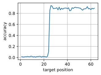
Probe: same model, patterns of length 24.

patterns of length 24: second-copy accuracy 0.02
attention mass at offset 31: 0.96
attention mass at offset 23: 0.00

• It learned look back exactly 31 positions — a RoPE offset head, no content, no matching.
• The qkv bias makes that head cheap: a constant, content-free query. Biases off — as in every model we analyze — the shortcut only half-forms.

A synthetic benchmark rewards the cheapest circuit it admits, not the mechanism its designer had in mind. Fix: make the period unpredictable.

Two blocks learn to look things up

Pattern length now uniform in 16–32; no fixed offset works.

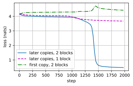
2 blocks: first copy 4.45, later copies 0.45, accuracy 0.87
1 block: first copy 4.31, later copies 3.67, accuracy 0.11

• Two blocks: later copies below half a nat, ~9 of 10 tokens right.
• One block: stuck above three nats — copying-style heads only.

The phase change

• Hundreds of steps hugging the one-block curve, then a drop of a couple of nats within one or two hundred steps.
• When it happens varies by seed and framework — we describe the shape, not the schedule. Same cliff as the “induction bump” in real LMs (Olsson et al., 2022).

Caught in the act

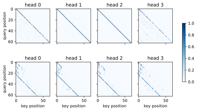
Block 1: a sharp line one step below the diagonal — a previous-token head. Block 2: a stripe at offset L-1, starting where the second copy starts — the induction stripe.

Scoring every head

Average mass on the previous token vs. on the induction target j = i + 1 - L:

block 1: previous token 0.02 0.01 0.92 0.03 | induction target 0.01 0.00 0.00 0.01
block 2: previous token 0.04 0.04 0.04 0.04 | induction target 0.62 0.68 0.69 0.49

• Previous-token attention lives in block 1, induction attention in block 2 — never the other way around. Which head does what varies by seed.

Pattern completion is in-context learning

Every evaluation pattern is new — no pair it copies was ever in training. The weights store an algorithm, not associations:

One exposure suffices; the restart itself is unpredictable in principle.

The circuit is in the weights

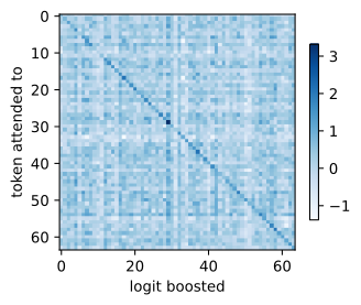
If block 2 copies, attending to token a should boost logit a: C_{ab} = \mathbf{e}_b^\top \mathbf{W}_{\mathrm{OV}} \mathbf{e}_a should be diagonal-dominant — checkable without a forward pass:

rows whose largest entry is the diagonal: 0.77 (chance 1/64)

What attention weights do not tell you

• Weights answer where, never what: the effect runs through OV — a sharp head can move nothing, a diffuse one can compute precisely.
• Different weights, same predictions (Jain & Wallace, 2019); the rebuttal (Wiegreffe & Pinter, 2019) sharpened, not settled, the debate.
• Our identification used behavior (the loss split), causal probes (period shift, ablation), and weight-level checks (the OV diagonal) — the stripes only said where to look.

In full transformers (FFN, LayerNorm, superposition) each step becomes a research problem: mechanistic interpretability. A handful of circuits — induction heads first — are understood at this level. Most are not.

Recap

• Residual stream: embeddings in, logits out, heads only add — this section’s vocabulary returns when we assemble full transformer blocks.
• Every head = QK circuit (where) × OV circuit (what), both rank d_h.
• Depth ladder: bigrams → skip-trigrams → induction (needs composition).
• Trained on repetition, TinyCharLM finds the induction circuit in a phase change; a fixed-period task is solved by a positional shortcut instead.
• Pattern completion over never-seen tokens = in-context learning in miniature — the mechanism implicated in LLM in-context learning.