The Cost of Attention

Dive into Deep Learning · §10.5

The cost of attention
the quadratic bill, measured · online softmax and FlashAttention · sliding windows · linear attention is an RNN

The bargain and the bill

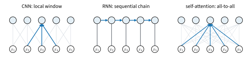
Map n tokens of dimension d to n tokens of dimension d:

layer complexity sequential ops max path length
convolution (k) \mathcal{O}(knd^2) \mathcal{O}(1) \mathcal{O}(n/k)
recurrence \mathcal{O}(nd^2) \mathcal{O}(n) \mathcal{O}(n)
self-attention \mathcal{O}(n^2d) \mathcal{O}(1) \mathcal{O}(1)

Full parallelism and constant path length — paid for by the one quadratic entry.

The quadratic bill, measured

One layer: 4n^2d FLOPs, two n \times n score buffers = 8n^2 bytes (fp32), per head, per sequence. Dominates the layer as soon as n > 2d.

n =  2048: XLA temp    32.0 MiB, predicted 8n^2 B =    32.0 MiB
n =  4096: XLA temp   128.0 MiB, predicted 8n^2 B =   128.0 MiB
n =  8192: XLA temp   512.0 MiB, predicted 8n^2 B =   512.0 MiB
n = 16384: XLA temp  2048.0 MiB, predicted 8n^2 B =  2048.0 MiB
  • Exact from n = 4096 up (the smallest run adds a few MiB of allocator overhead); doubling n quadruples the bill.
  • At n = 131{,}072: one fp32 attention map \approx 69 GB. Nobody stores it.

Time tells the same story

def wall_clock(f, *args, reps=10):
    f(*args).block_until_ready()  # Warm up (and compile)
    start = time.time()
    for _ in range(reps):
        f(*args).block_until_ready()
    return (time.time() - start) / reps

layer = jax.jit(attention_layer)
for n in [2048, 4096, 8192, 16384]:
    Q = jax.random.normal(jax.random.key(0), (n, d_h))
    print(f'n = {n:5d}: {wall_clock(layer, Q, Q, Q)*1e3:6.2f} ms')
n =  2048:   0.16 ms
n =  4096:   0.37 ms
n =  8192:   1.37 ms
n = 16384:   4.99 ms
  • Launch-bound while the GPU is idle; from a few thousand tokens on, each doubling of n roughly quadruples the time — 4n^2d in action.

Online softmax: the matrix never needs to exist

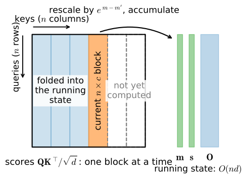
Per query, carry a running max, normalizer, and output; process keys in blocks:

m' = \max(m, \max_j a_j), \quad s' = s\,e^{m-m'} + \sum_j e^{a_j - m'}, \quad \mathbf{o}' = \mathbf{o}\,e^{m-m'} + \sum_j e^{a_j-m'}\mathbf{v}_j

\mathbf{o}/s is exactly \mathrm{softmax}(\mathbf{a})\mathbf{V} — raising the max retroactively rescales the past.

Chunked attention: exact, in linear memory

Twenty lines carry the update over all queries, one key block at a time:

n, d_h = 2048, 64
Q, K, V = (jax.random.normal(k, (n, d_h))
           for k in jax.random.split(jax.random.key(0), 3))
with jax.default_matmul_precision('highest'):
    err = jnp.abs(chunked_attention(Q, K, V)
                  - causal_attention(Q, K, V)).max()
print(f'maximum deviation: {float(err):.2e}')
maximum deviation: 4.62e-07
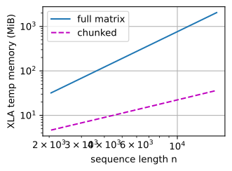
  • Same answer, same FLOPs; the n^2 footprint is gone.

The bottleneck is memory traffic, not FLOPs

GPUs multiply hundreds of times faster than they fetch. Naive attention writes n^2 scores to slow memory and reads them back twice. FlashAttention (Dao et al., 2022): tiles in on-chip SRAM, softmax stats in registers, backward pass recomputes instead of storing.

B, H, n = 2, 8, 8192
X = jax.random.normal(jax.random.key(0), (B, n, H, d_h), dtype=jnp.float16)

def naive_heads(X):
    Xt = X.transpose(0, 2, 1, 3)
    i = jnp.arange(X.shape[1])
    scores = Xt @ Xt.swapaxes(-1, -2) / math.sqrt(X.shape[-1])
    scores = jnp.where(i[None, :] > i[:, None],
                       jnp.finfo(scores.dtype).min, scores)
    return (jax.nn.softmax(scores, axis=-1) @ Xt).transpose(0, 2, 1, 3)

def fused_heads(X):
    return jax.nn.dot_product_attention(X, X, X, is_causal=True,
                                        implementation='cudnn')

for name, f in [('naive', naive_heads), ('fused', fused_heads)]:
    jitted = jax.jit(f)
    temp = jitted.lower(X).compile().memory_analysis().temp_size_in_bytes
    print(f'{name}: {wall_clock(jitted, X)*1e3:6.2f} ms, '
          f'XLA temp {temp/2**20:7.1f} MiB')
naive:   9.86 ms, XLA temp  4096.0 MiB
fused:   1.38 ms, XLA temp     0.0 MiB
  • Exact attention, an order of magnitude faster, quadratic buffer gone — ship it: scaled_dot_product_attention / jax.nn.dot_product_attention.

Attention through a window

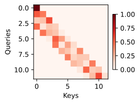
Let each query attend to the w most recent positions — the causal mask becomes a band:

  • \mathcal{O}(nw) work instead of \mathcal{O}(n^2).
  • Deployed: Mistral 7B (w = 4096, 32 layers); Longformer adds global tokens; NSA learns the sparsity pattern itself.

Depth restores the reach

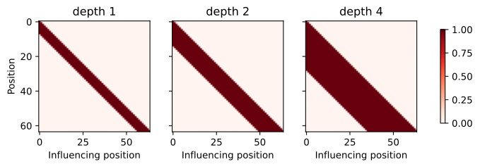
Information hops w-1 positions per layer: receptive field 1 + L(w-1) after L layers — computed, not asserted:

depth 1: last query reaches 8 positions (formula: 8)
depth 2: last query reaches 15 positions (formula: 15)
depth 4: last query reaches 29 positions (formula: 29)
  • The CNN bet (ch. 7), re-made: locality compounds through depth.

Linear attention: kernelize the score

Choose a factorizing kernel \phi(\mathbf{q})^\top\phi(\mathbf{k}) instead of \exp(\mathbf{q}^\top\mathbf{k}/\sqrt{d}). The query factors out of the attention sum:

\mathbf{o}_t = \frac{\phi(\mathbf{q}_t)^\top \mathbf{S}_t}{\phi(\mathbf{q}_t)^\top \mathbf{z}_t}, \qquad \mathbf{S}_t = \mathbf{S}_{t-1} + \phi(\mathbf{k}_t)\,\mathbf{v}_t^\top

A recurrent network: fixed d \times d matrix state, outer-product writes, queried like an associative memory (Katharopoulos et al., 2020; fast weight programmers, 1991).

Two forms, one answer

Parallel form (cumulative sums) for training; recurrent form (carry \mathbf{S}, \mathbf{z}) for generation:

n = 512
Q, K, V = (jax.random.normal(k, (n, d_h))
           for k in jax.random.split(jax.random.key(0), 3))
err = jnp.abs(linear_attention_parallel(Q, K, V)
              - linear_attention_recurrent(Q, K, V)).max()
print(f'maximum deviation: {float(err):.2e}')
print(f'recurrent state: {d_h}x{d_h} + {d_h} floats '
      f'= {(d_h * d_h + d_h) * 4 / 1024:.0f} KiB at any sequence length')
maximum deviation: 2.38e-07
recurrent state: 64x64 + 64 floats = 16 KiB at any sequence length
  • 16 KiB of state at any context length, vs. a KV cache that grows forever. The price: \mathbf{S}_t is a lossy summary of the past.

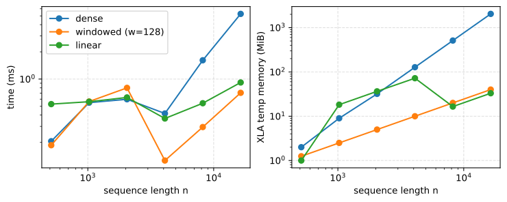
The price of attention, measured

  • Dense bends to slope 2; windowed hugs the launch floor; linear pays nd_h^2 memory and bandwidth-bound cumsums — its decisive win is the constant-memory recurrent mode.
  • The approximation zoo (Performer, Linformer, Reformer) is history: what survived is exact-but-clever, windowed, and linear-as-recurrence.

Recap: three ways out

  • Reorganize: online softmax → FlashAttention. Exact, linear memory; the bottleneck was traffic, not FLOPs.
  • Restrict: sliding windows; depth restores reach as 1 + L(w-1).
  • Kernelize: linear attention = linear recurrence with matrix state:

\mathbf{S}_t = \mathbf{S}_{t-1} + \phi(\mathbf{k}_t)\,\mathbf{v}_t^\top

That recurrence is the state-space recurrence of ch. 12 with identity decay; train it with the parallel scan, gate it and you get Mamba — attention and recurrence are two ends of one design space (SSD, 2024).