Self-Attention and Positional Encoding
Self-Attention
Bahdanau attention links two sequences (decoder steps to encoder steps). What if we use the same trick within a single sequence — let every token query every other token? That’s self-attention : queries, keys, and values all come from the same input.
The output for each token is a weighted average of all tokens, with weights determined by query-key compatibility. This is the elementary block of every Transformer encoder and decoder layer.
from d2l import jax as d2lfrom flax import linen as nnfrom jax import numpy as jnpimport jax
Reuse multi-head attention with the same input fed three times. Output shape matches input shape — same sequence length, same hidden size:
= 100 , 5 = d2l.MultiHeadAttention(num_hiddens, num_heads, 0.5 )
Shape check:
= 2 , 4 , d2l.tensor([3 , 2 ])= d2l.ones((batch_size, num_queries, num_hiddens))= False )[0 ][0 ],
CNN vs. RNN vs. self-attention
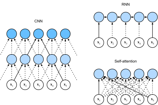
Three ways to map a length-n sequence to another length-n sequence with d -dim tokens:
CNN (k -wide)
\mathcal{O}(knd^2) \mathcal{O}(1) \mathcal{O}(n/k)
RNN
\mathcal{O}(nd^2) \mathcal{O}(n) \mathcal{O}(n)
Self-attention
\mathcal{O}(n^2 d) \mathcal{O}(1) \mathcal{O}(1)
Self-attention wins on parallelism and path length — every token reaches every other in one hop. The price is n^2 scaling.
One picture
CNN, RNN, self-attention. Path lengths: \mathcal{O}(n/k) , \mathcal{O}(n) , \mathcal{O}(1) .
Why we need positional encoding
Self-attention is permutation-equivariant: shuffle the input tokens, and the outputs shuffle the same way. The model has no idea about word order.
Solution: inject position information into each token’s representation. Vaswani et al. use fixed sine/cosine encodings:
p_{i,2j} = \sin\!\left(\frac{i}{10000^{2j/d}}\right),\quad p_{i,2j+1} = \cos\!\left(\frac{i}{10000^{2j/d}}\right).
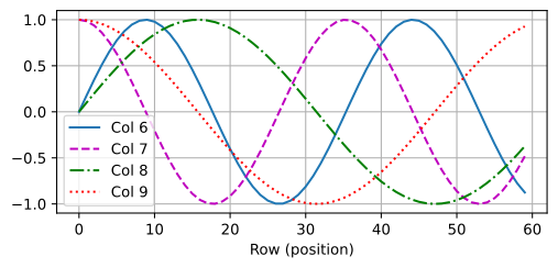
Different frequencies along the embedding dimension; same position i across all dims gives a unique fingerprint.
PositionalEncoding class
Precompute \mathbf{P} once for max_len positions, slice to actual length at forward time, add to inputs:
class PositionalEncoding(nn.Module):"""Positional encoding.""" int float int = 1000 def setup(self ):# Create a long enough P self .P = d2l.zeros((1 , self .max_len, self .num_hiddens))= d2l.arange(self .max_len, dtype= jnp.float32).reshape(- 1 , 1 ) / jnp.power(10000 , jnp.arange(0 , self .num_hiddens, 2 , dtype= jnp.float32) / self .num_hiddens)self .P = self .P.at[:, :, 0 ::2 ].set (jnp.sin(X))self .P = self .P.at[:, :, 1 ::2 ].set (jnp.cos(X[:, :self .num_hiddens // 2 ]))@nn.compact def __call__ (self , X, training= False , offset= 0 ):# Flax sow API is used to capture intermediate variables self .sow('intermediates' , 'P' , self .P)# `offset` lets autoregressive decoders advance the encoding position # past tokens already emitted, instead of always slicing from 0. = X + self .P[:, offset:offset + X.shape[1 ], :]return nn.Dropout(self .dropout)(X, deterministic= not training)
Frequency along the dimension
Plot four columns of \mathbf{P} . Lower-index columns oscillate fast; higher columns oscillate slow:
= 32 , 60 = PositionalEncoding(encoding_dim, 0 )= pos_encoding.init(d2l.get_key(), d2l.zeros((1 , num_steps, encoding_dim)))= pos_encoding.apply (params, d2l.zeros((1 , num_steps, encoding_dim)),= 'intermediates' )= inter_vars['intermediates' ]['P' ][0 ] # retrieve intermediate value P = P[:, :X.shape[1 ], :]0 , :, 6 :10 ].T, xlabel= 'Row (position)' ,= (6 , 2.5 ), legend= ["Col %d " % d for d in range (6 , 10 )])
Position as continuous binary
Compare with binary representations of small integers — same “low bits flip fast, high bits flip slow” pattern, but in continuous values:
0 in binary is 000
1 in binary is 001
2 in binary is 010
3 in binary is 011
4 in binary is 100
5 in binary is 101
6 in binary is 110
7 in binary is 111
The full positional matrix
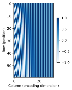
Heatmap reveals the multi-frequency structure. Each row is a unique fingerprint for a position:
Why sin/cos: relative positions
For any fixed offset \delta , the encoding at position i + \delta is a linear function of the encoding at position i :
\begin{bmatrix} p_{i+\delta, 2j} \\ p_{i+\delta, 2j+1} \end{bmatrix} =
\begin{bmatrix} \cos(\delta\omega_j) & \sin(\delta\omega_j) \\ -\sin(\delta\omega_j) & \cos(\delta\omega_j) \end{bmatrix}
\begin{bmatrix} p_{i, 2j} \\ p_{i, 2j+1} \end{bmatrix}.
The rotation depends on \delta but not on i . So the network can learn to “shift attention by 5 tokens” with one linear transformation — relative positions come for free.
Recap
Self-attention = multi-head attention with \mathbf{Q} = \mathbf{K} = \mathbf{V} = \mathbf{X} .
Output sequence length = input sequence length.
Compared to RNNs: same complexity per step but \mathcal{O}(1) path length and full parallelism. Cost: \mathcal{O}(n^2 d) .
Self-attention is permutation-equivariant; need positional encoding to know token order.
Sin/cos encoding gives unique absolute positions and lets the model express relative offsets as linear maps.