Statistics

Estimator Quality

A primer on the language of estimators that ML borrows heavily from:

• Estimator — a procedure that takes data and outputs a guess (e.g. sample mean, MLE).
• Bias — \mathbb{E}[\hat\theta] - \theta. Systematic error.
• Variance — \text{Var}(\hat\theta). Noise across datasets.
• MSE = bias^2 + variance — the basic decomposition that explains overfitting and why regularization helps.

This deck makes the bias-variance tradeoff concrete.

Evaluating estimators

An estimator is judged by its sampling distribution: repeat the same experiment on fresh datasets and ask where the estimates center and how widely they vary.

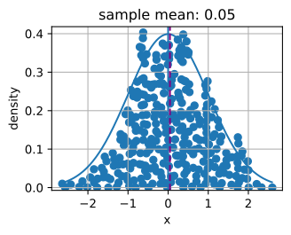
from d2l import jax as d2l
import jax
from jax import numpy as jnp
import numpy as np

# Sample datapoints and create y coordinate
epsilon = 0.1
key = jax.random.PRNGKey(8675309)
xs = jax.random.normal(key, (300,))

ys = jnp.array(
    [jnp.sum(jnp.exp(-(xs[:i] - xs[i])**2 / (2 * epsilon**2))
             / jnp.sqrt(2*jnp.pi*epsilon**2)) / len(xs)
     for i in range(len(xs))])

# Compute true density
xd = jnp.arange(jnp.min(xs), jnp.max(xs), 0.01)
yd = jnp.exp(-xd**2/2) / jnp.sqrt(2 * jnp.pi)

# Plot the results
d2l.plot(xd, yd, 'x', 'density')
d2l.plt.scatter(xs, ys)
d2l.plt.axvline(x=0)
d2l.plt.axvline(x=float(jnp.mean(xs)), linestyle='--', color='purple')
d2l.plt.title(f'sample mean: {float(jnp.mean(xs)):.2f}')
d2l.plt.show()

Empirical bias / variance

Simulate a sampling distribution: many datasets → many estimates → empirical mean and spread:

# Statistical bias
def stat_bias(true_theta, est_theta):
    return(jnp.mean(est_theta) - true_theta)

# Mean squared error
def mse(data, true_theta):
    return(jnp.mean(jnp.square(data - true_theta)))

theta_true = 1
sigma = 4
sample_len = 10000
key = jax.random.PRNGKey(0)
samples = jax.random.normal(key, (sample_len, 1)) * sigma + theta_true
theta_est = jnp.mean(samples)
theta_est

Array(0.98958063, dtype=float32)

Empirical bias / variance (cont.)

The second pass turns simulated estimates into empirical bias, variance, and MSE, making the bias-variance decomposition visible.

mse(samples, theta_true)

Array(16.385305, dtype=float32)

bias = stat_bias(theta_true, theta_est)
jnp.square(jnp.std(samples)) + jnp.square(bias)

Array(16.385307, dtype=float32)

A Gaussian example

Sample mean for \mathcal{N}(\mu, \sigma^2): unbiased, variance \sigma^2/n. Concretely visualize this:

# Number of samples
N = 1000

# Sample dataset
key = jax.random.PRNGKey(0)
samples = jax.random.normal(key, (N,))

# Lookup Students's t-distribution c.d.f.
t_star = 1.96

# Construct interval
mu_hat = jnp.mean(samples)
sigma_hat = jnp.std(samples, ddof=1)
(mu_hat - t_star*sigma_hat/jnp.sqrt(N), \
 mu_hat + t_star*sigma_hat/jnp.sqrt(N))

(Array(-0.06360511, dtype=float32), Array(0.05844307, dtype=float32))

Recap

• Estimator quality = bias + variance.
• Sample mean is BLUE for \mu — best linear unbiased estimator under iid Gaussian noise.
• Regularization trades a bit of bias for a lot of variance reduction.
• Same trade-off shows up everywhere: dropout, weight decay, ensembling.