Looking at the data

Naive Bayes

Naive Bayes Classification

Naive Bayes — the simplest probabilistic classifier. Apply Bayes’ rule:

P(y \mid \mathbf{x}) \propto P(y) \prod_i P(x_i \mid y).

The “naive” part is the assumption that features are conditionally independent given the class. Wrong in general — pixels of an image are obviously correlated — but the model is fast, requires little data, and is a useful starting point.

This deck applies it to MNIST digit classification with binarized pixels.

Setup + binary MNIST

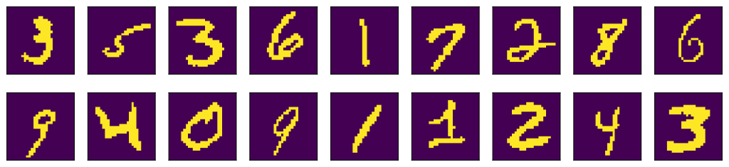
Binarize pixels so each pixel can be modeled as a Bernoulli random variable conditioned on the digit class.

%matplotlib inline
from d2l import jax as d2l
import math
import jax
from jax import numpy as jnp
import numpy as np
import tensorflow as tf
d2l.use_svg_display()

Inspect the binarized digits before fitting: the class templates are recognizable, but neighboring pixels are clearly dependent.

(train_images, train_labels), (
    test_images, test_labels) = tf.keras.datasets.mnist.load_data()
train_images = np.floor(train_images / 128).astype(np.float32)
test_images = np.floor(test_images / 128).astype(np.float32)
train_labels = train_labels.astype(np.int32)
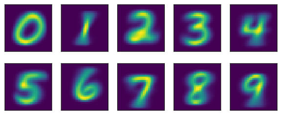
test_labels = test_labels.astype(np.int32)

image, label = train_images[2], train_labels[2]
image.shape, label

((28, 28), np.int32(4))

image.shape, image.dtype

((28, 28), dtype('float32'))

Per-class pixel statistics

For each class y and pixel i, estimate P(x_i = 1 \mid y) from the training set. With Laplace smoothing to avoid zeros:

label, type(label)

(np.int32(4), numpy.int32)

images = jnp.array(train_images[10:38])
labels = jnp.array(train_labels[10:38])
images.shape, labels.shape

((28, 28, 28), (28,))

d2l.show_images(images, 2, 9);

Training: just count

Training is counting, not gradient descent: estimate class priors and per-pixel likelihoods directly from the labeled examples.

X = jnp.array(train_images)
Y = jnp.array(train_labels)

n_y = jnp.zeros(10)
for y in range(10):
    n_y = n_y.at[y].set((Y == y).sum())
P_y = n_y / n_y.sum()
P_y

Array([0.09871667, 0.11236667, 0.0993    , 0.10218333, 0.09736667,
       0.09035   , 0.09863333, 0.10441667, 0.09751666, 0.09915   ],      dtype=float32)

n_x = jnp.zeros((10, 28, 28))
for y in range(10):
    n_x = n_x.at[y].set(
        jnp.array(np.array(X)[np.array(Y) == y].sum(axis=0)))
P_xy = (n_x + 1) / (n_y + 2).reshape(10, 1, 1)

d2l.show_images(P_xy, 2, 5);

Training (cont.)

Training stores only class priors and per-class pixel probabilities; prediction multiplies those likelihood terms, usually in log-space.

def bayes_pred(x):
    x = jnp.expand_dims(x, axis=0)  # (28, 28) -> (1, 28, 28)
    p_xy = P_xy * x + (1 - P_xy)*(1 - x)
    p_xy = p_xy.reshape(10, -1).prod(axis=1)  # p(x|y)
    return p_xy * P_y

image, label = test_images[0], test_labels[0]
bayes_pred(image)

Array([0., 0., 0., 0., 0., 0., 0., 0., 0., 0.], dtype=float32)

a = 0.1
print('underflow:', a**784)
print('logarithm is normal:', 784*math.log(a))

underflow: 0.0
logarithm is normal: -1805.2267129073316

Predicting in log-space

Sums of logs instead of products of probabilities — avoids underflow:

log_P_xy = jnp.log(P_xy)
log_P_xy_neg = jnp.log(1 - P_xy)
log_P_y = jnp.log(P_y)

def bayes_pred_stable(x):
    x = jnp.expand_dims(x, axis=0)  # (28, 28) -> (1, 28, 28)
    p_xy = log_P_xy * x + log_P_xy_neg * (1 - x)
    p_xy = p_xy.reshape(10, -1).sum(axis=1)  # p(x|y)
    return p_xy + log_P_y

py = bayes_pred_stable(image)
py

Array([-268.97256, -301.70444, -245.19516, -218.87387, -193.457  ,
       -206.09085, -292.52264, -114.62566, -220.33133, -163.17844],      dtype=float32)

jnp.argmax(py, axis=0) == label

Array(True, dtype=bool)

Evaluating

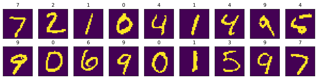
The accuracy is useful mostly as a sanity check: on images, the conditional-independence assumption leaves visible performance on the table.

def predict(X):
    return [int(jnp.argmax(bayes_pred_stable(x), axis=0)) for x in X]

X = jnp.array(test_images[:18])
y = jnp.array(test_labels[:18])
preds = predict(X)
d2l.show_images(X, 2, 9, titles=[str(d) for d in preds]);

X = jnp.array(test_images)
y = jnp.array(test_labels)
preds = jnp.array(predict(X), dtype=jnp.int32)
float((preds == y).sum()) / len(y)  # Validation accuracy

0.8427

Recap

• Bayes rule + conditional independence = naive Bayes.
• Training is one pass over the data — count and smooth.
• Surprisingly competitive baseline for text classification (sparse features, large vocab).
• Bad on images (independence is too wrong) — but a great teaching example for Bayesian classification.