Multivariable Calculus

Calculus in Many Dimensions

Generalize differentiation to many inputs. The gradient

\nabla f(\mathbf{x}) = [\partial f/\partial x_1, \ldots, \partial f/\partial x_d]^\top

points in the direction of steepest ascent; -\nabla f is the descent direction. Local quadratic structure is captured by the Hessian \nabla^2 f, the matrix of second partials.

The deck also covers the chain rule in vector form, and connects it to backpropagation — backprop is just reverse-mode application of the multivariate chain rule.

Higher-dimensional differentiation

Partial derivatives measure one coordinate at a time; the gradient bundles them into the vector pointing across level sets.

%matplotlib inline
from d2l import jax as d2l
from IPython import display
from mpl_toolkits import mplot3d
import jax
from jax import numpy as jnp
import numpy as np

def f(x, y):
    return jnp.log(jnp.exp(x) + jnp.exp(y))
def grad_f(x, y):
    return jnp.array([jnp.exp(x) / (jnp.exp(x) + jnp.exp(y)),
                      jnp.exp(y) / (jnp.exp(x) + jnp.exp(y))])

epsilon = jnp.array([0.01, -0.03])
grad_approx = f(jnp.array([0.]), jnp.log(
    jnp.array([2.]))) + jnp.dot(
    epsilon, grad_f(jnp.array([0.]), jnp.log(jnp.array(2.))))
true_value = f(jnp.array([0.]) + epsilon[0], jnp.log(
    jnp.array([2.])) + epsilon[1])
f'approximation: {grad_approx}, true Value: {true_value}'

'approximation: [1.0819457], true Value: [1.0821242]'

Optimization in many dimensions

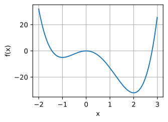
GD: \mathbf{x} \leftarrow \mathbf{x} - \eta \nabla f(\mathbf{x}). Newton: \mathbf{x} \leftarrow \mathbf{x} - [\nabla^2 f]^{-1} \nabla f. The latter is exact for quadratics, expensive in high dim:

x = jnp.arange(-2, 3, 0.01)
f = (3 * x**4) - (4 * x**3) - (12 * x**2)

d2l.plot(x, f, 'x', 'f(x)')

Chain rule and backprop

Reverse-mode auto-diff = walk the chain rule from outputs to inputs, accumulating partial derivatives:

# Compute the value of the function from inputs to outputs
w, x, y, z = -1, 0, -2, 1
a, b = (w + x + y + z)**2, (w + x - y - z)**2
u, v = (a + b)**2, (a - b)**2
f = (u + v)**2
print(f'    f at {w}, {x}, {y}, {z} is {f}')

# Compute the single step partials
df_du, df_dv = 2*(u + v), 2*(u + v)
du_da, du_db, dv_da, dv_db = 2*(a + b), 2*(a + b), 2*(a - b), -2*(a - b)
da_dw, db_dw = 2*(w + x + y + z), 2*(w + x - y - z)

# Compute the final result from inputs to outputs
du_dw, dv_dw = du_da*da_dw + du_db*db_dw, dv_da*da_dw + dv_db*db_dw
df_dw = df_du*du_dw + df_dv*dv_dw
print(f'df/dw at {w}, {x}, {y}, {z} is {df_dw}')

    f at -1, 0, -2, 1 is 1024
df/dw at -1, 0, -2, 1 is -4096

# Compute the value of the function from inputs to outputs
w, x, y, z = -1, 0, -2, 1
a, b = (w + x + y + z)**2, (w + x - y - z)**2
u, v = (a + b)**2, (a - b)**2
f = (u + v)**2
print(f'f at {w}, {x}, {y}, {z} is {f}')

# Compute the derivative using the decomposition above
# First compute the single step partials
df_du, df_dv = 2*(u + v), 2*(u + v)
du_da, du_db, dv_da, dv_db = 2*(a + b), 2*(a + b), 2*(a - b), -2*(a - b)
da_dw, db_dw = 2*(w + x + y + z), 2*(w + x - y - z)
da_dx, db_dx = 2*(w + x + y + z), 2*(w + x - y - z)
da_dy, db_dy = 2*(w + x + y + z), -2*(w + x - y - z)
da_dz, db_dz = 2*(w + x + y + z), -2*(w + x - y - z)

# Now compute how f changes when we change any value from output to input
df_da, df_db = df_du*du_da + df_dv*dv_da, df_du*du_db + df_dv*dv_db
df_dw, df_dx = df_da*da_dw + df_db*db_dw, df_da*da_dx + df_db*db_dx
df_dy, df_dz = df_da*da_dy + df_db*db_dy, df_da*da_dz + df_db*db_dz

print(f'df/dw at {w}, {x}, {y}, {z} is {df_dw}')
print(f'df/dx at {w}, {x}, {y}, {z} is {df_dx}')
print(f'df/dy at {w}, {x}, {y}, {z} is {df_dy}')
print(f'df/dz at {w}, {x}, {y}, {z} is {df_dz}')

f at -1, 0, -2, 1 is 1024
df/dw at -1, 0, -2, 1 is -4096
df/dx at -1, 0, -2, 1 is -4096
df/dy at -1, 0, -2, 1 is -4096
df/dz at -1, 0, -2, 1 is -4096

# Define the function to differentiate
def f_comp(w, x, y, z):
    a, b = (w + x + y + z)**2, (w + x - y - z)**2
    u, v = (a + b)**2, (a - b)**2
    return ((u + v)**2).squeeze()

w, x, y, z = jnp.array([-1.]), jnp.array([0.]), jnp.array([-2.]), jnp.array([1.])

# Compute gradients with respect to all four arguments
grad_f = jax.grad(f_comp, argnums=(0, 1, 2, 3))
w_grad, x_grad, y_grad, z_grad = grad_f(w, x, y, z)

print(f'df/dw at {w}, {x}, {y}, {z} is {w_grad}')
print(f'df/dx at {w}, {x}, {y}, {z} is {x_grad}')
print(f'df/dy at {w}, {x}, {y}, {z} is {y_grad}')
print(f'df/dz at {w}, {x}, {y}, {z} is {z_grad}')

df/dw at [-1.], [0.], [-2.], [1.] is [-4096.]
df/dx at [-1.], [0.], [-2.], [1.] is [-4096.]
df/dy at [-1.], [0.], [-2.], [1.] is [-4096.]
df/dz at [-1.], [0.], [-2.], [1.] is [-4096.]

Hessians

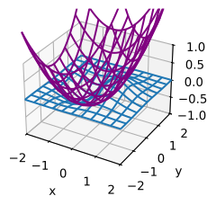
Curvature in many dimensions. PSD Hessian = local minimum, mixed signs = saddle, NSD = maximum:

# Construct grid and compute function
x, y = jnp.meshgrid(jnp.linspace(-2, 2, 101),
                     jnp.linspace(-2, 2, 101), indexing='ij')

z = x * jnp.exp(- x**2 - y**2)

# Compute approximating quadratic with gradient and Hessian at (1, 0)
w = jnp.exp(jnp.array([-1.])) * (-1 - (x + 1) + (x + 1)**2 + y**2)

# Plot function
ax = d2l.plt.figure().add_subplot(111, projection='3d')
ax.plot_wireframe(np.array(x), np.array(y), np.array(z),
                  **{'rstride': 10, 'cstride': 10})
ax.plot_wireframe(np.array(x), np.array(y), np.array(w),
                  **{'rstride': 10, 'cstride': 10}, color='purple')
d2l.plt.xlabel('x')
d2l.plt.ylabel('y')
d2l.set_figsize()
ax.set_xlim(-2, 2)
ax.set_ylim(-2, 2)
ax.set_zlim(-1, 1)
ax.dist = 12

Recap

• Gradient: direction of steepest ascent.
• Hessian: local curvature matrix; eigenvalues classify stationary points.
• Backprop = reverse-mode chain rule, \mathcal{O}(\text{model size}) per parameter.
• Same calculus everywhere: GD, Newton, conjugate gradient, Adam — they’re all approximations to the local Taylor expansion of the loss.