Maximum Likelihood

Maximum Likelihood

Maximum likelihood: pick the parameters that make the observed data most probable.

\hat\theta = \arg\max_\theta \prod_i p(x_i \mid \theta) = \arg\min_\theta -\sum_i \log p(x_i \mid \theta).

The negative log-likelihood form is what every classification and regression loss in the book actually optimizes:

  • Cross-entropy = NLL of a categorical p(y \mid x).
  • MSE = NLL of a Gaussian p(y \mid x) with fixed variance.
  • BPR / softmax-with-temperature etc. — all NLLs.

So “minimize the loss” is “do MLE” in fancy clothes.

A concrete example

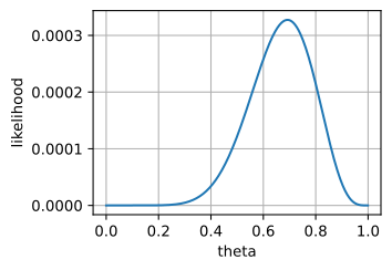
For 9 heads and 4 tails, the likelihood curve peaks at \hat\theta = 9/13: the observed fraction of heads.
%matplotlib inline
from d2l import jax as d2l
from jax import numpy as jnp

theta = jnp.arange(0, 1, 0.001)
p = theta**9 * (1 - theta)**4.

d2l.plot(theta, p, 'theta', 'likelihood')

Numerical optimization (NLL)

Sums of logs are easier than products: floating point behaves; gradients have closed forms; SGD works on the NLL.

import jax

# Set up our data
n_H = 8675309
n_T = 256245

# Initialize our parameters
theta = jnp.float32(0.5)

# Define loss function
def nll(theta):
    return -(n_H * jnp.log(theta) + n_T * jnp.log(1 - theta))

grad_fn = jax.grad(nll)

# Perform gradient descent
lr = 1e-9
for iter in range(100):
    theta = theta - lr * grad_fn(theta)

# Check output
theta, n_H / (n_H + n_T)
(Array(0.9713101, dtype=float32), 0.9713101437890875)

Recap

  • MLE: maximize \sum_i \log p(x_i \mid \theta); equivalently, minimize NLL.
  • Connects optimization (the chapter’s main topic) to probability (this chapter’s main topic).
  • Most “losses” in DL are NLLs of suitable conditional distributions.
  • MLE is consistent and asymptotically efficient for well-specified models.