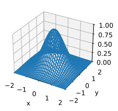
# Construct grid and compute function
x, y = jnp.meshgrid(jnp.linspace(-2, 2, 101), jnp.linspace(-2, 2, 101),
                     indexing='ij')
z = jnp.exp(- x**2 - y**2)

# Plot function
ax = d2l.plt.figure().add_subplot(111, projection='3d')
ax.plot_wireframe(x, y, z)
d2l.plt.xlabel('x')
d2l.plt.ylabel('y')
d2l.plt.xticks([-2, -1, 0, 1, 2])
d2l.plt.yticks([-2, -1, 0, 1, 2])
d2l.set_figsize()
ax.set_xlim(-2, 2)
ax.set_ylim(-2, 2)
ax.set_zlim(0, 1)
ax.dist = 12Geometric interpretation
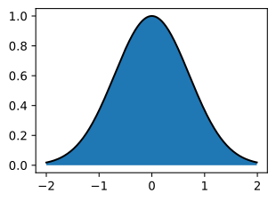
Integration starts as area under a nonnegative curve:
Definite integral
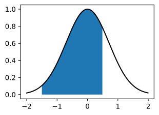
Most useful integrals are over an interval [a,b]:
\int_a^b f(x)\,dx.
Geometrically this keeps only the area between the vertical boundaries.
Riemann approximation
Approximate the area by rectangles; refine the partition; the limit is the integral.
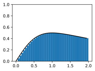
'approximation: 0.7944856882095337, truth: [0.804719]'Multiple integrals
\iint f(x, y)\, dA — total under a 2D surface; iterated integration treats one axis at a time: