Bernoulli

Distributions

Common Probability Distributions

A reference tour of the distributions used throughout the book — what they look like, when they apply, and how to sample / evaluate them in code.

• Bernoulli — single coin flip; binary classification conditional.
• Discrete uniform — equiprobable categories.
• Continuous uniform — random initialization, dropout masks (in expectation).
• Binomial — count of successes in n Bernoullis.
• Poisson — rare events count; CTR distributions, click counts.
• Gaussian — by far the most-used; CLT, regression noise model, default prior.

Setup

Imports and plotting helpers are shared across the PMF, PDF, CDF, and sampling examples below.

%matplotlib inline
from d2l import jax as d2l
from IPython import display
from math import erf, factorial
import jax
from jax import numpy as jnp
import numpy as np

P(X=1) = p, P(X=0) = 1-p. Mean p, variance p(1-p):

p = 0.3

d2l.set_figsize()
d2l.plt.stem([0, 1], [1 - p, p])
d2l.plt.xlabel('x')
d2l.plt.ylabel('p.m.f.')
d2l.plt.show()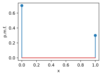

x = jnp.arange(-1, 2, 0.01)

def F(x):
    return 0 if x < 0 else 1 if x > 1 else 1 - p

d2l.plot(x, jnp.array([F(y) for y in x]), 'x', 'c.d.f.')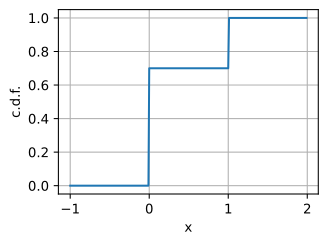

jax.random.bernoulli(jax.random.PRNGKey(0), p, shape=(10, 10)).astype(
    jnp.float32)

Array([[0., 0., 0., 0., 0., 1., 0., 0., 0., 1.],
       [0., 1., 0., 0., 0., 0., 0., 0., 0., 1.],
       [1., 0., 0., 0., 0., 0., 0., 0., 1., 1.],
       [1., 0., 0., 0., 0., 0., 0., 1., 0., 0.],
       [1., 1., 0., 0., 0., 1., 0., 1., 0., 0.],
       [0., 0., 1., 0., 0., 0., 1., 0., 1., 0.],
       [0., 0., 1., 0., 0., 1., 1., 0., 1., 0.],
       [0., 0., 0., 0., 0., 0., 1., 0., 0., 0.],
       [1., 0., 0., 0., 0., 0., 0., 0., 0., 0.],
       [1., 0., 0., 1., 0., 0., 0., 1., 0., 1.]], dtype=float32)

Discrete uniform

Equally likely categories. Maximum entropy on a finite set with no prior knowledge:

n = 5

d2l.plt.stem([i+1 for i in range(n)], n*[1 / n])
d2l.plt.xlabel('x')
d2l.plt.ylabel('p.m.f.')
d2l.plt.show()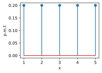

x = jnp.arange(-1, 6, 0.01)

def F(x):
    return 0 if x < 1 else 1 if x > n else jnp.floor(x) / n

d2l.plot(x, jnp.array([F(y) for y in x]), 'x', 'c.d.f.')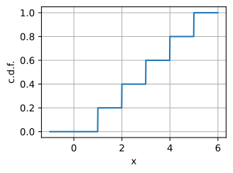

jax.random.randint(jax.random.PRNGKey(0), (10, 10), 1, n)

Array([[2, 1, 1, 2, 4, 4, 1, 4, 2, 4],
       [1, 3, 1, 4, 4, 4, 3, 3, 3, 2],
       [4, 1, 1, 4, 2, 2, 1, 2, 1, 1],
       [2, 1, 2, 4, 2, 3, 4, 1, 4, 1],
       [1, 4, 3, 4, 2, 3, 2, 3, 1, 4],
       [1, 4, 3, 2, 3, 3, 4, 4, 3, 3],
       [4, 2, 2, 2, 1, 3, 1, 3, 4, 3],
       [1, 1, 2, 2, 3, 1, 4, 1, 2, 2],
       [4, 1, 4, 3, 3, 2, 2, 3, 4, 2],
       [2, 1, 1, 1, 3, 3, 3, 4, 4, 4]], dtype=int32)

Continuous uniform

Density \frac{1}{b-a} on [a, b]. Source of pseudo-random samples for Monte Carlo and dropout:

a, b = 1, 3

x = jnp.arange(0, 4, 0.01)
p = (x > a).astype(jnp.float32) * (x < b).astype(jnp.float32) / (b - a)
d2l.plot(x, p, 'x', 'p.d.f.')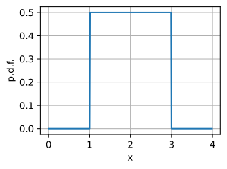

def F(x):
    return 0 if x < a else 1 if x > b else (x - a) / (b - a)

d2l.plot(x, jnp.array([F(y) for y in x]), 'x', 'c.d.f.')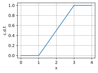

jax.random.uniform(jax.random.PRNGKey(0), (10, 10), minval=a, maxval=b)

Array([[2.895334 , 2.9571598, 1.664583 , 1.9373369, 2.1397774, 1.331006 ,
        1.6203892, 2.378961 , 2.4935331, 1.3420291],
       [2.9707077, 1.0505652, 2.2800837, 2.1253817, 2.7984276, 2.869075 ,
        2.6682804, 2.4512324, 2.0197062, 1.0553043],
       [1.0629776, 2.9160376, 2.0376384, 2.5844283, 2.1044838, 2.2227058,
        2.786351 , 2.5099819, 1.4232836, 1.4586995],
...
       [2.7144866, 2.247558 , 2.33837  , 2.7587452, 2.6359684, 2.7785282,
        1.5847943, 2.6081705, 1.9936442, 2.3641   ],
       [1.267415 , 2.9917667, 2.6263065, 2.6803617, 2.2014291, 2.0994458,
        2.755646 , 2.1530125, 1.8485291, 1.6624053],
       [1.2517128, 2.1566439, 2.7574615, 1.3824458, 2.6221197, 1.7307668,
        1.8838031, 1.3609681, 2.8293433, 1.4353452]], dtype=float32)

Binomial

Sum of n iid Bernoullis. Bell-shaped for large n (Gaussian limit):

from scipy.special import gammaln as lgamma

n, p = 10, 0.2

def log_binom_pmf(n, k, p):
    """Compute log(binom(n,k) * p^k * (1-p)^(n-k)) stably."""
    return (lgamma(n+1) - lgamma(k+1) - lgamma(n-k+1)
            + k * np.log(p) + (n-k) * np.log(1-p))

pmf = jnp.array([np.exp(log_binom_pmf(n, i, p)) for i in range(n + 1)])

d2l.plt.stem([i for i in range(n + 1)], pmf)
d2l.plt.xlabel('x')
d2l.plt.ylabel('p.m.f.')
d2l.plt.show()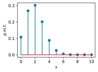

x = jnp.arange(-1, 11, 0.01)
cmf = jnp.cumsum(pmf)

def F(x):
    return 0 if x < 0 else 1 if x > n else cmf[int(x)]

d2l.plot(x, jnp.array([F(y) for y in x.tolist()]), 'x', 'c.d.f.')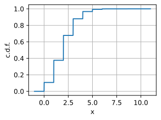

# JAX doesn't have a built-in binomial sampler, so we sum Bernoulli trials
jax.random.bernoulli(jax.random.PRNGKey(0), p, shape=(10, 10, n)).sum(axis=-1)

Array([[2, 2, 1, 1, 2, 1, 3, 0, 1, 3],
       [2, 1, 1, 2, 3, 3, 2, 4, 3, 1],
       [0, 3, 1, 0, 3, 3, 2, 0, 3, 2],
       [3, 2, 2, 3, 2, 0, 4, 2, 1, 3],
       [2, 0, 3, 0, 2, 1, 2, 1, 3, 2],
       [1, 1, 5, 1, 1, 2, 2, 0, 3, 0],
       [1, 0, 2, 2, 1, 1, 0, 3, 1, 2],
       [1, 2, 2, 1, 3, 4, 2, 3, 3, 1],
       [4, 1, 1, 2, 4, 0, 0, 3, 1, 3],
       [0, 1, 2, 2, 1, 2, 2, 5, 6, 2]], dtype=int32)

Poisson

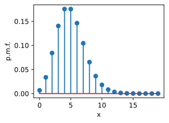
Rare events: P(X = k) = \frac{\lambda^k e^{-\lambda}}{k!}. Approximates binomial with n large, p small, np \to \lambda:

Poisson CDF

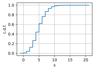
The cumulative distribution sums the probability of observing up to k events:

F(k)=P(X \le k).

Poisson samples

Sampling turns the distribution into count data: nonnegative integers with mean and variance both near \lambda.

Array([[ 1,  2,  5,  5,  3,  3,  4,  8,  2,  5],
       [ 2,  6,  5,  4,  5,  5,  1,  4,  2,  2],
       [ 7,  4,  3,  4,  6,  2,  4,  5,  4,  6],
       [ 6,  5,  6,  5,  4,  4,  1,  2,  4,  3],
       [ 2,  1,  3,  6, 11,  9,  8,  7,  3,  5],
       [11,  2,  7,  6,  3,  1,  3,  9,  7,  6],
       [ 3,  5,  3,  4,  5,  6,  7,  5,  5,  3],
       [ 3,  4,  6,  7,  6,  4,  7,  3,  5,  4],
       [ 4,  2,  6,  8,  4,  7,  3,  5,  5,  5],
       [ 5,  8,  5,  2,  6,  4,  5,  3,  7,  8]], dtype=int32)

Gaussian

\mathcal{N}(\mu, \sigma^2) — bell curve. CLT makes it the limit of many small contributions; that’s why it’s everywhere:

p = 0.2
ns = [1, 10, 100, 1000]
d2l.plt.figure(figsize=(10, 3))
for i in range(4):
    n = ns[i]
    pmf = jnp.array([np.exp(log_binom_pmf(n, i, p))
                      for i in range(n + 1)])
    d2l.plt.subplot(1, 4, i + 1)
    d2l.plt.stem([(i - n*p)/np.sqrt(n*p*(1 - p))
                  for i in range(n + 1)], pmf)
    d2l.plt.xlim([-4, 4])
    d2l.plt.xlabel('x')
    d2l.plt.ylabel('p.m.f.')
    d2l.plt.title("n = {}".format(n))
d2l.plt.show()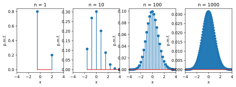

mu, sigma = 0, 1

x = jnp.arange(-3, 3, 0.01)
p = 1 / jnp.sqrt(2 * jnp.pi * sigma**2) * jnp.exp(
    -(x - mu)**2 / (2 * sigma**2))

d2l.plot(x, p, 'x', 'p.d.f.')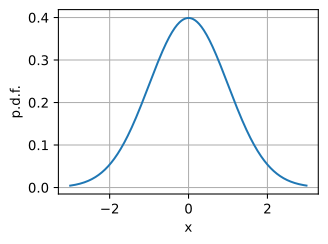

Gaussian (cont.)

Changing \mu shifts the bell curve; changing \sigma spreads it. Samples concentrate near the mean and thin out in the tails.

def phi(x):
    return (1.0 + erf((x - mu) / (sigma * jnp.sqrt(2.)))) / 2.0

d2l.plot(x, jnp.array([phi(y) for y in x.tolist()]), 'x', 'c.d.f.')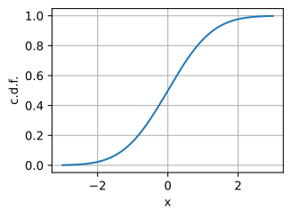

mu + sigma * jax.random.normal(jax.random.PRNGKey(0), (10, 10))

Array([[ 1.6226422 ,  2.0252647 , -0.43359444, -0.07861735,  0.1760909 ,
        -0.97208923, -0.49529874,  0.4943786 ,  0.6643493 , -0.9501635 ],
       [ 2.1795304 , -1.9551506 ,  0.35857072,  0.15779513,  1.2770847 ,
         1.5104648 ,  0.970656  ,  0.59960806,  0.0247007 , -1.9164772 ],
       [-1.8593491 ,  1.728144  ,  0.04719035,  0.814128  ,  0.13132767,
         0.28284705,  1.2435943 ,  0.6902801 , -0.80073744, -0.74099   ],
...
       [ 1.0680159 ,  0.31542128,  0.43766403,  1.1718564 ,  0.9077099 ,
         1.2226242 , -0.54639524,  0.85630435, -0.00796578,  0.47343913],
       [-1.1090349 ,  2.6423514 ,  0.88957626,  0.9952015 ,  0.2551972 ,
         0.12496138,  1.164173  ,  0.19296366, -0.19099544, -0.43659472],
       [-1.1461989 ,  0.19760251,  1.1686655 , -0.8733985 ,  0.8818086 ,
        -0.3441057 , -0.14614972, -0.91352165,  1.370097  , -0.7800775 ]],      dtype=float32)

Recap

• A small toolkit covers most needs: Bernoulli, uniform (discrete/continuous), binomial, Poisson, Gaussian.
• CLT makes the Gaussian central — sums of many small effects look Gaussian.
• Each distribution has a closed-form NLL → standard loss in DL.