Density evolution under stochastic dynamics Fokker–Planck, the probability-flow ODE, and the reverse SDE.
From stochastic paths to deterministic densities
Motivation
An SDE path is random, whereas its time-marginal density p_t(\mathbf x) evolves deterministically.
Drift transports it, diffusion smooths it.
The same marginals can be produced by a deterministic ODE.
The reverse SDE and probability-flow ODE both require the score\nabla\log p_t.
01
From paths to densities
the two viewpoints and the vector-calculus toolkit
Marginals average over path randomness
Two viewpoints
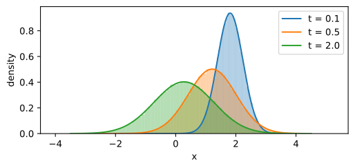
The Lagrangian view follows one realization; the Eulerian view tracks the time-marginal p_t(\mathbf x), which averages over all noise and is therefore reproducible. A hundred thousand OU walkers land on the analytic Gaussians:
t=0.1: cloud mean +1.8121 (analytic +1.8097), std 0.4275 (analytic 0.4258)
t=0.5: cloud mean +1.2137 (analytic +1.2131), std 0.7987 (analytic 0.7951)
t=2.0: cloud mean +0.2750 (analytic +0.2707), std 0.9889 (analytic 0.9908)
Three facts from vector calculus
The toolkit
Divergence\nabla\cdot\mathbf v: net flux per unit volume.
Laplacian\Delta h: how far h sits below its neighborhood average.
By parts\int h\,(\nabla\cdot\mathbf v) = -\int \nabla h\cdot\mathbf v.
These three identities suffice for the derivations that follow.
02
The Fokker–Planck equation
derivation, term reading, the OU check
Itô + by parts → a PDE
Derivation
For a test function \phi, Itô’s lemma gives d\phi=(\nabla\phi\cdot\mathbf f+\tfrac12 g^2\Delta\phi)dt+\text{noise}. Take \mathbb E[\cdot]=\int(\cdot)\,p_t, use the zero mean of the Itô integral, and integrate by parts onto p_t:
For \mathbf f = -\nabla V and constant g, this PDE is itself a gradient flow: steepest descent of the free energy \int pV + \tfrac12 g^2\!\int p\log p in the Wasserstein geometry (Jordan–Kinderlehrer–Otto), the same transport geometry used by flow matching.
Drift transports, diffusion smooths
Reading the PDE
-\nabla\cdot(\mathbf f p) streams probability along the drift; \tfrac12 g^2\Delta p raises p wherever it dips below its neighborhood. With \mathbf f=\mathbf 0 it is the heat equation, variance growing linearly.
The Ornstein–Uhlenbeck check
A closed-form solution
A Gaussian \mathcal N(m(t),v(t)) solves the OU Fokker–Planck iff
\dot m = -\theta m, \qquad \dot v = \sigma^2 - 2\theta v
(match coefficients of (x-m)^0,(x-m)^1,(x-m)^2). The steady state gives \mathcal N(0,\sigma^2/2\theta); numerically the residual is tiny:
def ou_density(x, t, x0=2.0): m, v = ou_mean_var(x0, t)return np.exp(-(x - m)**2/ (2* v)) / np.sqrt(2* np.pi * v)xs = np.linspace(-4.0, 5.0, 4001)dx = xs[1] - xs[0]for t in ts_show: eps =1e-5 dpdt = (ou_density(xs, t + eps) - ou_density(xs, t - eps)) / (2* eps) p = ou_density(xs, t) transport = np.gradient(theta * xs * p, dx) # -d/dx(f p), f = -theta x diffusion =0.5* sigma**2* np.gradient(np.gradient(p, dx), dx) residual = (dpdt - (transport + diffusion))[5:-5] # trim one-sided edge stencilsprint(f't={t}: max|residual| = {np.abs(residual).max():.2e}, 'f'max|dp/dt| = {np.abs(dpdt).max():.2e}')
Under the stated positivity, regularity, boundary, and well-posedness assumptions, this ODE has the same time-marginals as the SDE. Invertibility and the likelihood identity additionally concern the exact field and exact integration.
SDE and ODE marginals
The experiment
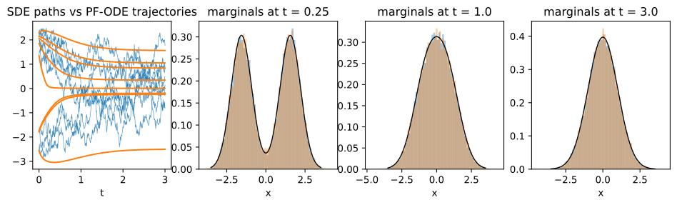
Same target marginals, different motion: SDE paths cross while ODE trajectories are smooth and do not cross under uniqueness. In this finite experiment the empirical CDF gap remains below 0.009:
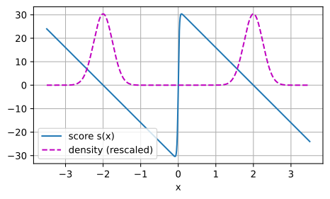
\mathbf s_t(\mathbf x)=\nabla_{\mathbf x}\log p_t(\mathbf x) points uphill on the log-density and vanishes at every interior critical point. Curvature distinguishes modes from troughs and saddles. Gaussian: -(\mathbf x-\boldsymbol\mu)/\sigma^2, a spring to the mean; a mixture gives responsibility-weighted springs.
Scores remove the normalizing constant
Normalizer-invariance
For p=\tilde p/Z, \nabla\log p = \nabla\log\tilde p since \nabla\log Z = 0. An energy model p\propto e^{-E} has score -\nabla E, no intractable Z:
A network can represent the score without evaluating Z. This removes one obstacle; estimation error, support, and integrability still matter.
05
Time reversal
Anderson’s theorem and the factor of two
Anderson’s reverse-time SDE
Time reversal
Running the diffusion backward from the terminal Gaussian:
d\mathbf X = \bigl[\mathbf f - g(t)^2\,\nabla\log p_t(\mathbf X)\bigr]dt + g(t)\,d\bar{\mathbf W}.
A Bayesian Euler step shows why: the marginal p_t acts as a prior that bends each reversed step toward where the data was.
Reverse-time noise doubles the score correction at λ = 1
Time reversal
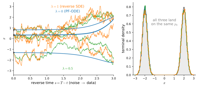
Within this scalar, state-independent diffusion family, one dial gives \mathbf b_\lambda = \mathbf f - \tfrac{1+\lambda^2}{2}g^2\nabla\log p_t with noise \lambda g, all sharing the marginals p_t. More injected noise, more drift correction: the factor slides from \tfrac12 g^2 (\lambda=0, the PF-ODE) to g^2 (\lambda=1, Anderson):
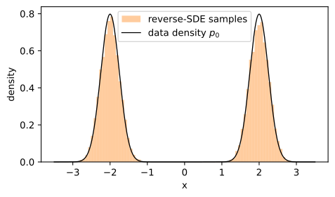
The exact mixture score recovers the bimodal target numerically
Generation
The closed-form mixture score isolates the reverse-SDE computation without training. A diffusion model replaces that analytic field with an estimate:
max|p_T - N(0,1)| at T=3: 0.0015  (vs peak 0.3974)
mass split: 0.500 / 0.500  (target 0.5 / 0.5)
left mode:  mean -1.999, std 0.260  (target -2.000, 0.250)
right mode: mean +2.001, std 0.261  (target +2.000, 0.250)
KS(generated, exact p0 sample) = 0.0172
Recap
Wrap-up
Fokker–Planck, \partial_t p = -\nabla\cdot(\mathbf f p)+\tfrac12 g^2\Delta p: drift transports, diffusion smooths.
Transport identity (plus sign!) makes it a continuity equation.
Under the stated regularity and boundary assumptions, the PF-ODE has the same marginals as the SDE; exact likelihood also requires exact integration.
Score \nabla\log p_t: normalizer-free and directed along log-density ascent.
Reverse SDE drift corrects by g^2\nabla\log p_t, twice the ODE’s.
When forward drift and diffusion are fixed, the score is the field to estimate.
Next: learn that score via score matching, diffusion, and flow matching.