Concise Implementation of Softmax Regression

Dive into Deep Learning · §3.5

Concise softmax regression
A linear layer with a numerically stable framework loss.

Same model, far fewer lines

Motivation

The from-scratch version built softmax, then log, then the negative-log-likelihood by hand. The concise version replaces all of it with two built-ins:

one linear layer in place of W and b;
one cross-entropy call that takes raw scores.

The convenience hides one thing: the loss is not the naive softmax → log → NLL. It is the stable rewrite.

The concise model

a linear layer in the Classifier scaffold

One linear layer, wrapped

The model

Flatten each image to a 784-vector, then a single linear layer to the 10 class scores. Everything else is inherited from Classifier:

class SoftmaxRegression(d2l.Classifier):
    """The softmax regression model."""
    def __init__(self, num_outputs, lr):
        super().__init__()
        self.save_hyperparameters()
        self.net = tf.keras.models.Sequential()
        self.net.add(tf.keras.layers.Flatten())
        self.net.add(tf.keras.layers.Dense(num_outputs))

    def forward(self, X):
        return self.net(X)

The forward pass returns logits

The model

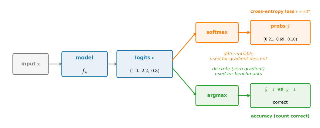
The forward method does not apply softmax. It returns raw scores \mathbf{o}\in\mathbb{R}^{10} (the logits).

Logits, not probabilities. The loss will own the softmax step. Applying softmax here and in the loss would apply it twice.

Why the loss is rewritten

overflow, underflow, and the log-sum-exp trick

Numerical instability in a direct softmax

Numerical stability

Softmax exponentiates the logits: \hat y_j = \exp(o_j) / \sum_k \exp(o_k).

Float32 spans roughly 10^{-38} to 10^{38}: \exp overflows to \infty once its argument passes \approx +88, and past \approx -88 it gradually underflows through the subnormals, hitting exactly 0 near -104.

Feed the from-scratch softmax the logits \mathbf{o}=(1000, 0, 0): \exp(1000)=\infty, the ratio is \infty/\infty= NaN, and a NaN propagates through the backward pass. The example in the softmax-from-scratch section; the fused loss below never forms that ratio.

Fix, step 1: shift by the max

Numerical stability

Softmax is unchanged if we subtract the same constant from every logit (the \exp\bar{o} factors cancel). Choose \bar{o}=\max_k o_k:

\hat y_j = \frac{\exp(o_j - \bar{o})}{\sum_k \exp(o_k - \bar{o})}, \qquad \bar{o} = \max_k o_k.

Now every exponent o_j - \bar{o} \le 0, so each \exp lands in (0, 1]: no overflow. The denominator sits in [1, q].

Fix, step 2: never form the softmax

Numerical stability

Underflow remains a problem if we then take \log of a near-zero probability. But we only ever want \log \hat y_j for the loss, so fold the \log in and the division disappears:

\log \hat y_j = (o_j - \bar{o}) - \log \sum_k \exp(o_k - \bar{o}).

No probability is materialized: the expression evaluates neither \exp of a large positive argument nor \log of an underflowed zero.

The log-sum-exp loss

Numerical stability

For true class y the loss \ell = -\log \hat y_y becomes a function of the logits alone:

\ell(y, \mathbf{o}) = \underbrace{\bar{o} + \log \textstyle\sum_k \exp(o_k - \bar{o})}_{\text{log-sum-exp, evaluated stably}} - o_y.

\log\sum_k\exp(o_k) is a smooth upper bound on \max_k o_k, which motivates the name soft maximum.

Its gradient is \partial_{o_j}\ell = \mathrm{softmax}(\mathbf{o})_j - y_j, with no clamp to perturb it.

The soft maximum differs by at most log 2

Numerical stability · the bound

For two classes with logits (x, 0) the loss’s first term is \mathrm{lse}(x, 0) = \log(1 + e^x), a smooth curve hugging \max(x, 0) from above:

\max_k o_k \;\le\; \mathrm{lse}(\mathbf{o}) \;\le\; \max_k o_k + \log q.

The gap peaks at the tie x = 0, where it equals \log 2 \approx 0.69, the bound \log q you proved in the softmax-regression section (exercise 6), here at q = 2. The gap decreases away from the tie.

In code

one fused call, four frameworks

Pass logits directly to the loss

The fused loss

SparseCategoricalCrossentropy(from_logits=True) is the switch that says “these are scores, not probabilities”, so Keras does the stable log-sum-exp instead of assuming a softmax already ran:

@d2l.add_to_class(d2l.Classifier)
def loss(self, Y_hat, Y, averaged=True):
    Y_hat = d2l.reshape(Y_hat, (-1, Y_hat.shape[-1]))
    Y = d2l.reshape(Y, (-1,))
    reduction = (tf.keras.losses.Reduction.SUM_OVER_BATCH_SIZE
                 if averaged else tf.keras.losses.Reduction.NONE)
    fn = tf.keras.losses.SparseCategoricalCrossentropy(
        from_logits=True, reduction=reduction)
    return fn(Y, Y_hat)

The fused-loss interface

The fused loss

The name differs by library; the interface does not. The built-in fused loss takes logits, not probabilities: passing softmax outputs would softmax twice.

Defined once on Classifier (note the #@save): the whole book inherits the stable loss.

Train

same linear model with framework components

Train

Results

Same Fashion-MNIST, same 10 epochs, same Trainer:

data = d2l.FashionMNIST(batch_size=256)
model = SoftmaxRegression(num_outputs=10, lr=0.1)
trainer = d2l.Trainer(max_epochs=10)
trainer.fit(model, data)

In the displayed run, validation accuracy is ~83–84%, close to the from-scratch model in the softmax-from-scratch section. The implementation uses a stable fused loss rather than explicit softmax followed by clipping.

Recap

Wrap-up

From scratch taught what softmax and cross-entropy are; concise uses the stable framework components typical of applications.
The forward pass outputs logits; the built-in loss owns the softmax.

That built-in is the log-sum-exp rewrite \ell = \bar{o} + \log\sum_k e^{o_k-\bar{o}} - o_y, not a naive softmax → log → NLL.
lse is a smooth max: within \log q of \max_k o_k, gap largest (\log 2 for q{=}2) exactly at the tie.
The fused expression avoids the float32 \pm 88 (and -104) thresholds by evaluating the stable log-sum-exp form directly.