An unpadded convolution with k>1shrinks its input. With an n \times n image and a k \times k kernel:
n \times n \;\longrightarrow\; (n - k + 1) \times (n - k + 1).
Stack ten 5×5 layers on a 240×240 image:
240 \to 236 \to 232 \to \ldots \to 200.
The output has 30% less area, with positions removed at the boundary. Padding controls this shrinkage; stride deliberately reduces the number of evaluated positions.
The boundary problem
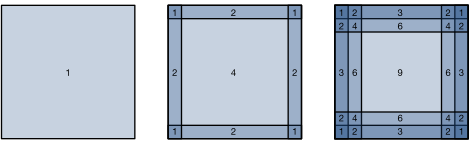
Even before stacking, single convs use boundary pixels much less than central ones. Each pixel only contributes when the kernel window covers it — interior pixels appear in many windows, whereas corner pixels appear in one:
Pixel utilization: 1×1, 2×2, and 3×3 kernels. Larger kernels make the boundary problem worse.
Boundary pixels contribute to fewer windows than interior pixels. Padding increases their participation and can preserve output shape, although the chosen boundary values still affect the result.
Padding: add zeros around the input
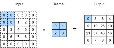
Add a “frame” of zero-valued pixels around the input. The kernel can now slide further, including positions where its window hangs off the original image:
3×3 input padded to 5×5; 2×2 kernel gives a 4×4 output. The shaded element is 0{\cdot}0 + 0{\cdot}1 + 0{\cdot}2 + 0{\cdot}3 = 0.
For odd k, (k-1)/2 is an integer, so we can pad symmetrically, the same on both sides, and the output position (i, j) corresponds to a window centered on input (i, j).
Even k forces a left/right asymmetry — pad floor on one side, ceil on the other.
This alignment is why odd kernels with symmetric padding are common in CNNs, for example 3×3 kernels with padding 1 and 7×7 kernels with padding 3.
Padding helper
Define a helper to wrap input/output reshaping, then ask the basic question: 8×8 input, 3×3 kernel, padding=1 — what’s the output shape?
import tensorflow as tf
Shape-preserving padding
# We define a helper function to calculate convolutions. It initializes# the convolutional layer weights and performs corresponding dimensionality# elevations and reductions on the input and outputdef comp_conv2d(conv2d, X):# (1, 1) indicates that batch size and the number of channels are both 1 X = tf.reshape(X, (1, ) + X.shape + (1, )) Y = conv2d(X)# Strip the first two dimensions: examples and channelsreturn tf.reshape(Y, Y.shape[1:3])# 1 row and column is padded on either side, so a total of 2 rows or columns# are addedconv2d = tf.keras.layers.Conv2D(1, kernel_size=3, padding='same')X = tf.random.uniform(shape=(8, 8))comp_conv2d(conv2d, X).shape
TensorShape([8, 8])
Same shape — the padded conv is “shape-preserving”. With an asymmetric kernel, mirror the asymmetry in the padding:
# We use a convolution kernel with height 5 and width 3. The padding on# either side of the height and width are 2 and 1, respectivelyconv2d = tf.keras.layers.Conv2D(1, kernel_size=(5, 3), padding='same')comp_conv2d(conv2d, X).shape
TensorShape([8, 8])
Stride: skipping positions on purpose
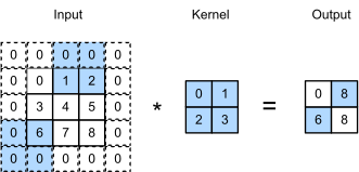
To reduce a large input, move the kernel by s > 1 at each step — skipping intermediate positions:
Cross-correlation with vertical stride 3 and horizontal stride 2. The kernel jumps three rows down and two columns right.
Computational benefit: s\times fewer positions to evaluate in each direction, so s_h s_w \times fewer operations. Statistical benefit: aggressive downsampling forces the network to summarize.
A more aggressive (and asymmetric) version — kernel 3×5, padding 0×1, stride 3×4:
# tf.keras.Conv2D accepts only 'same'/'valid' for `padding`; we use a# ZeroPadding2D layer to apply padding=(0, 1) (matching the MX/PT/JAX# tabs) before the convolution.conv2d = tf.keras.Sequential([ tf.keras.layers.ZeroPadding2D(padding=(0, 1)), tf.keras.layers.Conv2D(1, kernel_size=(3, 5), padding='valid', strides=(3, 4))])comp_conv2d(conv2d, X).shape
TensorShape([2, 2])
The output formula above predicts the shape; the code verifies it.
Dilation: nine weights, a wider view
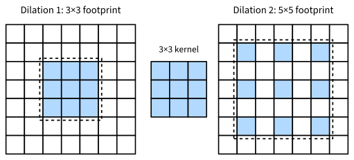
A dilated convolution spaces the kernel taps d pixels apart. Effective kernel size k + (k-1)(d-1): a 3×3 kernel at dilation 2 samples a 5×5 window at unchanged cost.
A 3×3 kernel at dilation 1 and dilation 2.
# Dilation 2 gives the 3x3 kernel a 5x5 footprint, so both convolutions# shrink the 8x8 input to 4x4conv2d = tf.keras.layers.Conv2D(1, kernel_size=3, padding='valid', dilation_rate=2)conv5 = tf.keras.layers.Conv2D(1, kernel_size=5, padding='valid')comp_conv2d(conv2d, X).shape, comp_conv2d(conv5, X).shape
(TensorShape([4, 4]), TensorShape([4, 4]))
Doubling d at every layer grows the receptive field exponentially with depth. Standard tool in dense prediction (FCN, DeepLab), where the output must keep full resolution.
Three patterns to remember
These three patterns occur frequently:
kernel
padding
stride
output
Preserve
3
1
1
n \times n
Halve
3
1
2
n/2 \times n/2
Patchify
k
0
k
n/k \times n/k
Preserve: ResNet feature mixing. Halve: standard downsample layer. Patchify: ViT turns 224×224 into a 14×14 grid of 16×16 patches in one shot.
Recap
An unpadded convolution shrinks: n \to n - k + 1. Cumulative shrinkage removes boundary positions.
Padding p grows the input — pick p = k - 1 to preserve shape (“SAME”). Odd kernels make this symmetric.
Stride s skips positions — s = 2 is the standard downsampler; large s patchifies.
Dilation d spreads the taps: effective kernel k + (k-1)(d-1), exponential receptive-field growth at fixed cost.
One formula covers all three: \text{out} = \Big\lfloor \frac{n - d(k-1) - 1 + p}{s} \Big\rfloor + 1.
Pad and stride per-axis; height and width are independent.