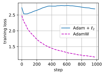
The comparison holds the model, tuned \eta, and \lambda = 0.1 fixed while changing coupled to decoupled decay:
curves = {}for name, opt_cls in [('Adam + $\\ell_2$', torch.optim.Adam), ('AdamW', torch.optim.AdamW)]: torch.manual_seed(0) model = d2l.TinyLM(len(data.vocab)) optimizer = opt_cls(model.parameters(), lr=0.003, weight_decay=0.1) curves[name] = d2l.train_lm(model, data, optimizer, num_steps=1000)d2l.plot(list(range(0, 1000, 25)), [smooth(c) for c in curves.values()],'step', 'training loss', legend=list(curves))
Decoupled: trains as if the decay were absent.
Coupled: stuck a full nat higher. Progress shrinks \sqrt{\hat{\mathbf{v}}} → the penalty comes back amplified; once it dominates, Adam normalizes it and increasing \lambda has little effect.
Learning-rate and decay sweeps
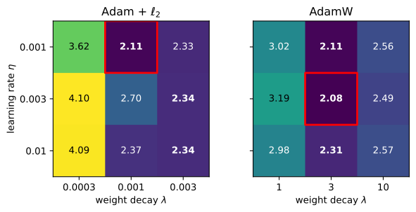
3\times 3 learning rate × weight decay, held-out loss, on a training slice small enough to overfit. Best \lambda per row in bold; each panel’s best cell boxed in red:
For AdamW, the best displayed \lambda is the same at every \eta, so the two hyperparameters can be searched more independently.
Coupled: the optimum wanders, and lives 2–3 orders of magnitude lower.
Fully tuned, both reach similar loss; decoupling makes the two hyperparameters easier to tune independently.
What weight decay is actually doing at scale
One-epoch LLM training has little classical overfitting, yet many reported configurations use \lambda = 0.1. Several scale-control effects help explain this choice.
Normalized layers are scale-invariant → gradient noise pushes norms up, decay pulls down → equilibrium: constant rotation per step (Kosson et al., 2024).
Through this equilibrium, \lambda influences the effective learning rate; decayed runs reach lower training loss, not a train/val trade (D’Angelo et al., 2024). Plus: keeps bf16 out of divergence.
\eta\lambda = a timescale: \tau = B/(\eta\lambda D) epochs; scale \lambda with B, D instead of re-tuning (Bergsma et al., 2025).
What not to decay
The census populations of §9.6, treated differently:
Matrices receive decay (96% of parameters).
Normalization parameters and biases are exempt because they directly set normalization scales.
Embeddings are exempt because their gradients are sparse while decay applies every step; OLMo 2 traced spikes to decay grinding embedding norms down (1/\|\mathbf{x}\| in LayerNorm’s gradient).
torch.manual_seed(0)model = d2l.TinyLM(len(data.vocab))decay = [p for name, p in model.named_parameters()if p.ndim ==2and'emb'notin name]no_decay = [p for name, p in model.named_parameters()if p.ndim !=2or'emb'in name]optimizer = torch.optim.AdamW([ {'params': decay, 'weight_decay': 0.1}, {'params': no_decay, 'weight_decay': 0.0}], lr=0.003)n_decay =sum(p.numel() for p in decay)n = n_decay +sum(p.numel() for p in no_decay)print(f'decayed: {n_decay} of {n} parameters')
decayed: 396800 of 412188 parameters
Section 9.9 uses the same matrix/non-matrix split: Muon assigns matrices a different optimizer rather than only a different decay setting.
Optimizer-state memory
AdamW stores two additional numbers per parameter:
                                           B/param    TinyLM  7B model
fp32 weights, grads, m, v                       16     6.6MB     112GB
bf16 weights + grads, fp32 master, m, v         16     6.6MB     112GB
the same + fp32 gradient accumulator            20     8.2MB     140GB
bf16 parameters still require an fp32 master copy in this configuration.
7B model ≈ 140 GB, 12 of 20 B/param is optimizer state.
Shrink it: Adafactor (factored v), 8-bit states. Or shard it: ZeRO (→ ch. 11, §29.6).
Recap
\ell_2 through Adam ≠ weight decay: the preconditioner changes \lambda per coordinate, backwards. AdamW decouples: one \lambda, one meaning.
Decoupled knobs tune separately: best \lambda independent of \eta in our grid.
At scale, decay = effective-LR control via the noise–decay equilibrium, on timescale 1/(\eta\lambda).