Dive into Deep Learning · §4.4
Numerical Stability and Initialization
Vanishing gradients, exploding gradients, and variance-preserving scales
Motivation
A deep network composes many layers. Its initial weights strongly affect the scale of forward activations and backward gradients.
Three ideas made deep training routine:
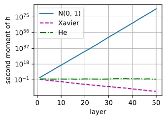
An unsuitable initialization can make gradients vanish or diverge before useful learning begins. In the examples below, ten sigmoid layers reduce the gradient to 10^{-6}; a hundred random matrices explode past 10^{24}; and one closing plot shows 10^{80} vs 10^{-15} vs flat (naive, Xavier, He).
01
Unstable Gradients
why the chain rule makes depth dangerous
Unstable Gradients
Backprop multiplies one Jacobian per layer. For a weight in layer \ell,
\partial_{\mathbf{W}^{(\ell)}} \mathbf{o} = \underbrace{\mathbf{M}^{(L)} \cdots \mathbf{M}^{(\ell+1)}}_{L-\ell \text{ Jacobians}}\, \mathbf{v}^{(\ell)}, \qquad \mathbf{M}^{(k)} = \partial_{\mathbf{h}^{(k-1)}} \mathbf{h}^{(k)}.
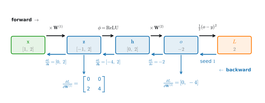
Forward pass builds z, h, o, L; the backward sweep multiplies a gradient back through every node.
Unstable Gradients
Whether the product grows or shrinks is set by the Jacobians’ scale.
A constant per-layer factor \rho compounds to \rho^{\,L-\ell}. Only \rho \approx 1 stays usable across depth.
Unstable Gradients · vanishing
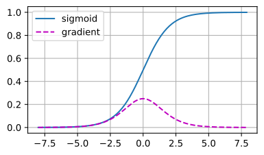
The sigmoid’s derivative peaks at 0.25 and is flat at zero in both tails.
Stack ten such layers and 0.25^{10} \approx 10^{-6}: the bottom layer sees a millionth of the gradient.
ReLU’s derivative is exactly 1 on active coordinates, so the activation does not attenuate gradients there. This property contributes to its use as a common default.
Unstable Gradients · exploding
Multiply one hundred \mathcal{N}(0,1) matrices (for i in range(100): M = M @ randn(4, 4)), exactly what a deep linear stack does to a gradient. The scale of each factor causes rapid growth in the product:
a single matrix
tensor([[ 1.0284, -1.3055, 1.1237, -0.5713],
[-1.6580, 0.1712, 0.8036, -0.0430],
[ 0.2606, 0.5971, -0.7985, -0.7436],
[ 1.0064, -0.7472, -0.8872, 0.4081]])
after multiplying 100 matrices
tensor([[-3.6839e+24, 1.6218e+26, 2.5680e+25, -5.4812e+25],
[ 1.8284e+24, -8.0495e+25, -1.2746e+25, 2.7205e+25],
[ 1.3880e+24, -6.1106e+25, -9.6755e+24, 2.0652e+25],
[-2.0169e+24, 8.8793e+25, 1.4059e+25, -3.0009e+25]])
A similarly scaled deep linear network produces gradients of unusable magnitude, for which ordinary optimization typically fails.
Unstable Gradients · in practice
Unstable Gradients · symmetry
Set every weight in a layer to the same constant c:
The h-unit layer therefore behaves like a single unit under gradient descent.
Gradient descent alone never breaks this tie. Random initialization does; so does dropout. Bias may still start at 0.
02
Variance-Preserving Init
keep the signal’s scale constant through depth
Initialization
For a linear layer o_i = \sum_{j=1}^{n_\textrm{in}} w_{ij} x_j with i.i.d. zero-mean weights (\textrm{Var} = \sigma^2) and inputs (\textrm{Var} = \gamma^2):
\mathbb{E}[o_i] = 0, \qquad \textrm{Var}[o_i] = n_\textrm{in}\, \sigma^2\, \gamma^2.
To carry the input’s variance through unchanged (\textrm{Var}[o] = \gamma^2), the only knob is \sigma^2:
\sigma^2 = \frac{1}{n_\textrm{in}}.
Initialization
The same variance count run backward through \mathbf{W}^\top sums over the n_\textrm{out} outputs instead:
\text{forward: } n_\textrm{in}\,\sigma^2 = 1 \qquad \text{backward: } n_\textrm{out}\,\sigma^2 = 1.
Both cannot hold at once unless n_\textrm{in} = n_\textrm{out}, so Xavier splits the difference by averaging the two fan sizes.
Preserve the activation scale on the way in and the gradient scale on the way out: one \sigma^2, two demands.
Initialization
Xavier / Glorot (2010), for \tanh and sigmoid:
\sigma^2 = \frac{2}{n_\textrm{in} + n_\textrm{out}}.
He / Kaiming (2015), for ReLU:
\sigma^2 = \frac{2}{n_\textrm{in}}.
ReLU zeroes half a symmetric signal, halving its second moment (E[\textrm{ReLU}(z)^2] = \tfrac{1}{2}E[z^2]), so He doubles the weight variance to compensate.
Rule of thumb: Xavier for \tanh/sigmoid, He for ReLU. Both ship as named initializers in most libraries.
Initialization · result
All three regimes in one plot: push a unit-scale signal through 50 ReLU layers and track E[(h^{(l)})^2] under three weight scales:
Beyond
A suitable initialization provides usable activation and gradient scales at the start of training. To reach hundreds of layers, modern architecture re-normalizes during training:
We return to both in the chapters on modern CNNs.
Wrap-up
Next (the generalization-in-deep-learning section): the model trains, but why does an over-parametrized network generalize at all?