Forward Propagation, Backward Propagation, and Computational Graphs

Dive into Deep Learning · §4.3

Forward and Backward Propagation
The chain rule on a computational graph

How a gradient is computed

Motivation

Training so far: a forward pass computes the loss, then one call to backward() returns every parameter gradient. This section makes that calculation explicit.

Forward: push the input through the net, storing each intermediate value.
Backward: walk the same graph in reverse, accumulating gradients by the chain rule.
The chain rule explains both the computation and its memory requirements.

The worked example computes all four gradients manually, and a short autograd script verifies the numerical values.

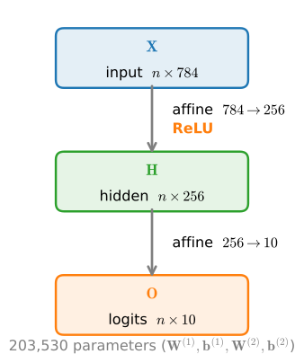
A one-hidden-layer MLP: input, an affine map, a nonlinearity, a second affine map.

Forward Propagation

computing and storing each intermediate value

The forward pass, one layer at a time

Forward Propagation

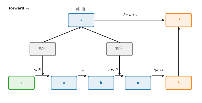
For input \mathbf{x}\in\mathbb{R}^d, a one-hidden-layer net (no bias, for clarity) computes a chain of intermediate variables:

\mathbf{z}= \mathbf{W}^{(1)}\mathbf{x}, \qquad \mathbf{h}= \phi(\mathbf{z}), \qquad \mathbf{o}= \mathbf{W}^{(2)}\mathbf{h}.

The loss is L = l(\mathbf{o}, y); the \ell_2 penalty is s = \tfrac{\lambda}{2}(\|\mathbf{W}^{(1)}\|_\textrm{F}^2 + \|\mathbf{W}^{(2)}\|_\textrm{F}^2).

The objective we actually minimize bundles both:

J = L + s.

Forward propagation as a graph

Forward Propagation

Squares are variables, circles are operators; arrows show data flow, running input (lower-left) to output (upper-right):

Computational graph of forward propagation: input and weights flow rightward and upward into the loss L, the regularizer s, and the objective J.

Every arrow is a dependency. The graph is the only thing the framework needs to record to later compute gradients.

Backpropagation

the same graph, traversed in reverse

Backpropagation applies the chain rule

Backpropagation

For \mathsf{Y}=f(\mathsf{X}) and \mathsf{Z}=g(\mathsf{Y}), the chain rule composes derivatives:

\frac{\partial \mathsf{Z}}{\partial \mathsf{X}} = \textrm{prod}\!\left(\frac{\partial \mathsf{Z}}{\partial \mathsf{Y}}, \frac{\partial \mathsf{Y}}{\partial \mathsf{X}}\right).

\textrm{prod} multiplies after any needed transpose or reshape: matrix multiplication for vectors, its tensor counterpart otherwise. It hides the bookkeeping so we can think one node at a time.

Backward through our network

Backpropagation

Seed \partial J/\partial L = \partial J/\partial s = 1 at the top, then walk back. Each step multiplies the incoming gradient by one local derivative:

\frac{\partial J}{\partial \mathbf{o}} = \frac{\partial L}{\partial \mathbf{o}}, \qquad \frac{\partial J}{\partial \mathbf{h}} = {\mathbf{W}^{(2)}}^\top\frac{\partial J}{\partial \mathbf{o}}, \qquad \frac{\partial J}{\partial \mathbf{z}} = \frac{\partial J}{\partial \mathbf{h}}\odot\phi'(\mathbf{z}).

The same reverse traversal produces the parameter gradients, including each weight-decay term:

\frac{\partial J}{\partial \mathbf{W}^{(2)}} = \frac{\partial J}{\partial \mathbf{o}}\,\mathbf{h}^\top + \lambda\mathbf{W}^{(2)}, \qquad \frac{\partial J}{\partial \mathbf{W}^{(1)}} = \frac{\partial J}{\partial \mathbf{z}}\,\mathbf{x}^\top + \lambda\mathbf{W}^{(1)}.

Gradients add at graph branches

Backpropagation

The “+” in \partial J/\partial \mathbf{W}^{(2)} encodes a general rule: \mathbf{W}^{(2)} reaches the objective along two paths, and the gradients arriving along each path sum:

J \leftarrow L \leftarrow \mathbf{o} \leftarrow \mathbf{W}^{(2)} \;\;(\text{the prediction path}), \qquad J \leftarrow s \leftarrow \mathbf{W}^{(2)} \;\;(\text{the regularizer path}).

Forgetting to accumulate at such forks (writing = where += belongs) is among the most common bugs in hand-written backward passes. Every autograd engine accumulates for exactly this reason.

Local backward rules

Backpropagation · local chain rule

Each backward step applies the same local rule: at each node, multiply the gradient arriving from downstream by the node’s local derivative.

Add node d = a + b
\partial d/\partial a = \partial d/\partial b = 1
→ passes the gradient through unchanged.

Multiply node e = d\,c
\partial e/\partial d = c,\ \partial e/\partial c = d
→ scales the gradient by the other input.

Every backward equation in this section applies this local rule.

A Worked Example

a numerical traversal of the graph

A tiny graph, by hand

Worked Example

Take e = (a+b)\,c at a=2,\ b=1,\ c=-3. Forward: d = a+b = 3, then e = d\,c = -9.

Backward: seed \partial e/\partial e = 1. The multiply node gives \partial e/\partial d = c = -3; the add node passes that through to both inputs:

\frac{\partial e}{\partial a} = -3,\qquad \frac{\partial e}{\partial b} = -3,\qquad \frac{\partial e}{\partial c} = d = 3.

An addition copies the incoming gradient; a multiplication scales it by the other input.

The forward pass, with numbers

Worked Example

Consider the network with d=h=2, q=1, ReLU activation, \lambda=0, squared-error loss, and

\mathbf{x}=\begin{bmatrix}1\\2\end{bmatrix},\quad \mathbf{W}^{(1)}=\begin{bmatrix}1&-1\\0&\phantom{-}1\end{bmatrix},\quad \mathbf{W}^{(2)}=[\,2\ \ {-1}\,],\quad y=0.

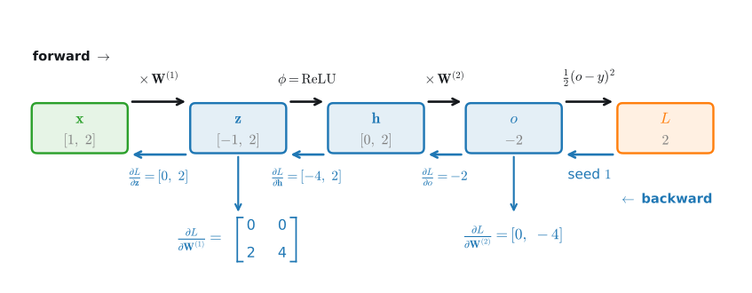
Pushing forward: \mathbf{z}=[-1,\,2]^\top, so \mathbf{h}=\phi(\mathbf{z})=[0,\,2]^\top (the first unit is dead), then o=-2 and L=2.

The backward sweep

Worked Example

Seed 1 at L, walk left. Add nodes pass the gradient, multiply nodes scale it; the dead ReLU unit (z_1=-1) zeros everything flowing into the top row of \mathbf{W}^{(1)}, so no signal means no learning.

Forward (black) carries values from \mathbf{x} to the loss L; backpropagation (blue) walks the same graph in reverse, multiplying each node’s local derivative to accumulate \partial L/\partial\mathbf{W}^{(2)} and \partial L/\partial\mathbf{W}^{(1)}. The dead first unit zeros the top row of \partial L/\partial\mathbf{W}^{(1)}.

The dying ReLU, made concrete

Worked Example

At the hidden layer, \phi'(z) = \mathbf{1}[z>0] acts as a gate:

\frac{\partial L}{\partial \mathbf{z}} = \frac{\partial L}{\partial \mathbf{h}}\odot\phi'(\mathbf{z}) = [-4,\,2]^\top \odot [0,\,1]^\top = [0,\,2]^\top.

So the parameter gradient is

\frac{\partial L}{\partial \mathbf{W}^{(1)}} = \frac{\partial L}{\partial \mathbf{z}}\,\mathbf{x}^\top = \begin{bmatrix}0&0\\2&4\end{bmatrix}.

The top row is all zero: the dead unit receives no gradient, so its weights never update. This is the dying ReLU in one matrix.

Verify the gradients with autograd

Worked Example · verified

Rebuild the same tensors with gradient tracking, run the forward pass, and sweep backward. The entire verification is a few lines:

x, y = torch.tensor([1., 2.]), 0
W1 = torch.tensor([[1., -1.], [0., 1.]], requires_grad=True)
W2 = torch.tensor([[2., -1.]], requires_grad=True)
z = W1 @ x
h = torch.relu(z)
o = W2 @ h
for v in (z, h): v.retain_grad()  # keep gradients of non-leaf tensors
L = ((o - y) ** 2).sum() / 2
L.backward()
print(f'L = {L.item()}, dL/dW2 = {W2.grad}, dL/dh = {h.grad}')
print(f'dL/dz = {z.grad}, dL/dW1 =\n{W1.grad}')

Autograd repeats every number

Worked Example · verified

The script compares autograd with the manual derivation:

L = 2.0, dL/dW2 = tensor([[-0., -4.]]), dL/dh = tensor([-4.,  2.])
dL/dz = tensor([0., 2.]), dL/dW1 =
tensor([[0., 0.],
        [2., 4.]])

L = 2.0,\quad \tfrac{\partial L}{\partial \mathbf{W}^{(2)}} = [0,\ {-4}],\quad \tfrac{\partial L}{\partial \mathbf{h}} = [-4,\ 2]^\top,\quad \tfrac{\partial L}{\partial \mathbf{z}} = [0,\ 2]^\top,\quad \tfrac{\partial L}{\partial \mathbf{W}^{(1)}} = \bigl[\begin{smallmatrix} 0 & 0\\ 2 & 4\end{smallmatrix}\bigr].

Every gradient matches, down to the zeroed row for the dead unit. (The -0 is floating point’s signed zero, h_1 = 0 times a negative upstream gradient; it compares equal to 0.)

Why It Matters

autograd, and the cost of remembering

From the chain rule to autograd

Why It Matters

The manual calculation follows the same procedure as backward(): record the graph on the forward pass, seed a 1 at the scalar loss, and sweep in reverse, multiplying each local derivative to accumulate every parameter gradient in a single pass.

This output-to-input sweep is reverse-mode automatic differentiation, cheap precisely when there are many parameters and one scalar loss: the deep-learning regime.

We developed the mechanics, including when forward mode is preferable, in the automatic-differentiation section; the full theory (both modes as Jacobian products and their memory trade-offs) is developed in the calculus appendix.

Forward and backward depend on each other

Why It Matters

The two passes are interlocked:

Forward uses the current parameters (set by the last backward step).
Backward reuses the stored intermediates \mathbf{h}, \mathbf{z}, \ldots from the forward pass.

So training alternates them, and must retain every intermediate until the backward pass consumes it.

That stored state is why training needs far more memory than prediction: it grows with depth and batch size, and is the usual cause of out-of-memory errors.

Recap

Wrap-up

Forward propagation computes and stores intermediates, input to output.
Backpropagation sweeps the same graph in reverse, accumulating gradients by the chain rule.
The local rules are simple: add passes the gradient and multiply scales it.

Gradients add at forks: a variable used twice collects both paths’ gradients (+=, never =).
A dead ReLU zeros a gradient row: no signal, no learning.
Autograd reproduced the hand derivation digit for digit.
Retaining intermediates is why training is memory-hungry.

Capstone (exercise 6): build a miniature autograd engine (a scalar Value class with +, *, relu and a topological backward()) and re-derive today’s example with it.