Naive Bayes

Dive into Deep Learning · §27.7

The chapter’s ideas at work in one system
count, smooth, argmax, then check the result.

Why not fit p(y | x) directly?

Motivation

A classifier wants \hat y = \operatorname{argmax}_y p(y\mid\mathbf x). An unrestricted conditional table has 2^d binary feature patterns and is impractical at MNIST scale (d=784).

The plan: maximum likelihood (the maximum-likelihood section) fits a generative model by counting; Bayes flips it into a classifier; the statistics of the statistics section then judge the result: error bar, failure map, calibration.

Bayes’ rule → a generative classifier

The route

Flip to the generative direction; the label-independent denominator drops:

\hat y = \operatorname*{argmax}_y\, p(y\mid\mathbf x) = \operatorname*{argmax}_y\, p(\mathbf x\mid y)\,p(y).

We still owe a model for p(\mathbf x\mid y), a distribution over all 2^d patterns. No savings yet.

Generative vs. discriminative

Two routes

Generative (here): learn class-conditionals p(\mathbf x\mid y) + prior, flip through Bayes.
Discriminative (softmax / logistic): fit the boundary p(y\mid\mathbf x) directly.

In some well-specified comparisons, generative fitting approaches its asymptotic error with fewer samples while discriminative fitting has lower asymptotic error. This ordering is model dependent.

The naive assumption

conditional independence, and why it helps

The factorization

Independence

Assume features are conditionally independent given the label:

p(\mathbf x\mid y) = \prod_{i=1}^d p(x_i\mid y).

For binary features, this replaces 2^d-1 class-conditional parameters per class by d Bernoulli parameters.

The graphical model

Independence

The label is a parent of every feature; no feature-to-feature edges appear in the factorized model. The right panel illustrates conditional dependence that the model does not represent.

For MNIST the assumption is inaccurate because pixels remain correlated within a class. Classification can still be useful even when probabilities are miscalibrated.

Log space and linearity

underflow, the log-sum, and Bernoulli decision boundaries

Predict in log space

Numerical

Multiplying 784 probabilities underflows: in single precision nearly every class score becomes an exact zero. Since \log is increasing it preserves the argmax and turns the product into a sum:

\hat y = \operatorname*{argmax}_y\, \log p(y) + \sum_{i=1}^d \log p(x_i\mid y).

Bernoulli scores are affine

Linearity

For binary pixels, \log p(x_i\mid y) = x_i\log p_{iy} + (1-x_i)\log(1-p_{iy}), so each class score is

s_y(\mathbf x) = \mathbf w_y^\top\mathbf x + b_y.

Naive Bayes draws the same kind of decision hyperplanes as softmax regression; only the way it fits the weights differs.

Gaussian naive Bayes is linear only when each feature variance is shared across classes; class-specific variances generally give quadratic boundaries.

Training is counting

priors, likelihoods, and Laplace smoothing

Maximum likelihood = frequencies

Counting

Both ingredients are counts: the class prior \hat p(y)=n_y/n and the per-pixel firing rate, Laplace-smoothed as \hat p(x_i{=}1\mid y) = \tfrac{n_{iy}+1}{n_y+2} so a never-seen pixel cannot send a log-score to -\infty:

n_y = np.array([(Y == y).sum() for y in range(10)])
P_y = n_y / n_y.sum()                                  # class prior, p(y)

n_x = np.stack([X[Y == y].sum(axis=0) for y in range(10)])
P_xy = (n_x + 1) / (n_y + 2).reshape(10, 1, 1)         # Laplace-smoothed p(x_i=1|y)
P_y

array([0.09871667, 0.11236667, 0.0993    , 0.10218333, 0.09736667,
       0.09035   , 0.09863333, 0.10441667, 0.09751667, 0.09915   ])

The +1/+2 is the posterior mean under a \text{Beta}(1,1) prior: pseudo-observations as regularization.

MNIST, end to end

binarize, learn templates, 84% accuracy

Load and binarize

MNIST

Threshold each 28\times28 grayscale image at 128 to get binary pixels x_i\in\{0,1\}:

def load(train):
    ds = torchvision.datasets.MNIST(root='../data', train=train, download=True)
    X = np.floor(ds.data.numpy() / 128).astype('float32')
    return X, ds.targets.numpy()

X, Y = load(train=True)
X_test, Y_test = load(train=False)
X.shape, Y.shape

((60000, 28, 28), (60000,))

A Gaussian naive Bayes would instead keep a per-class mean and variance for each continuous pixel.

What the model learns

MNIST

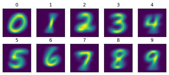
Each class is just an averaged template. The blur is the naive assumption: per-pixel marginals, nothing about co-occurrence.

d2l.show_images([P_xy[y] for y in range(10)], 2, 5,
                titles=[str(y) for y in range(10)]);

Classify and evaluate

MNIST

Sum the log-likelihoods, take the argmax, and measure what the raw products would have done:

float32 underflow: 99.1% of class scores; smallest float64 survivor = 1e-323
0.8427

84.27% on this implementation: far above 10\% chance and far below modern image classifiers. Conditional independence and binarization are both important model limitations.

A common domain: text

Domain

Pixels are tightly coupled. In a bag-of-words representation, the factorized model is often a useful and inexpensive baseline, including for spam filtering.

The multinomial event model counts word occurrences (with a +|V| denominator) instead of presence/absence.

Evaluation and uncertainty

error bar · failure map · calibration

How precise is 84.27%?

Error bar

Accuracy on 10,000 test examples is an estimate of population accuracy. A bootstrap interval quantifies its sampling uncertainty by resampling the test set and recomputing the statistic:

test accuracy = 0.8427, bootstrap 95% CI = (0.8354, 0.8496)

The 95% bootstrap interval is summarized as 84.3\%\pm0.7 percentage points, so reporting a third decimal is not meaningful. Comparing two models on the same test set requires a paired analysis; overlapping marginal intervals do not by themselves imply that their difference is insignificant.

Classwise errors

A confusion matrix identifies systematic confusions

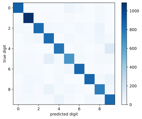
most confused true->predicted: 4->9 (138), 5->3 (106), 8->3 (68), 7->9 (67)

The largest confusions (4\to9, 5\to3, and 8\to3) occur among classes with similar learned templates. Distinguishing them depends partly on joint patterns among neighboring pixels, which the marginal feature model omits.

Calibration of posterior scores

Calibration

After normalization, the class scores define posterior probabilities under the fitted model. Calibration compares these probabilities with empirical frequencies by binning examples according to predicted confidence:

mean claimed confidence = 0.986,   actual accuracy = 0.843
confidence in (0.0, 0.9]:   447 examples,  claimed 0.7229,  achieved 0.3736
confidence in (0.9, 0.99]:   455 examples,  claimed 0.9606,  achieved 0.4747
confidence in (0.99, 0.999]:   406 examples,  claimed 0.9960,  achieved 0.5640
confidence in (0.999, 1.0]:  8692 examples,  claimed 1.0000,  achieved 0.8991

The mean predicted confidence is 98.6\%, while accuracy is 84.3\%. In the highest-confidence bin, predictions are correct 89.9\% of the time.

The model treats 784 correlated pixels as conditionally independent and therefore overcounts redundant evidence. The median gap between the largest and second-largest class scores is about 30 nats, enough to make the normalized posterior nearly degenerate. Probability estimates intended for downstream use should be checked with a calibration analysis.

Recap

Wrap-up

Naive Bayes combines Bayes’ rule with conditional feature independence.
For binary features, the factorization reduces an unrestricted 2^d-1-parameter class-conditional distribution to d Bernoulli parameters per class.
Parameter estimates are smoothed empirical counts, and prediction is performed in log space.
Bernoulli and multinomial scores are affine; Gaussian boundaries are linear only under shared per-feature variances and otherwise quadratic.

The method is often useful for sparse text features but is limited on images by conditional dependence and the chosen pixel likelihood.
This experiment obtains 84.3\%\pm0.7 accuracy. The confusion matrix identifies similar templates, and the calibration curve shows substantial overconfidence.

An accuracy report is more informative when accompanied by uncertainty, classwise errors, and a calibration check.