Numerical Stability and Conditioning
Dive into Deep Learning · §26.5
Numerical Stability and Conditioning
floating point · stable softmax · cancellation · conditioning
The math is right; the loss is NaN
Motivation
The preceding results assume real arithmetic, while a GPU uses a finite set of floating-point values. Two questions help locate a numerical error:
- Did the algorithm solve a nearby problem? (backward error)
- Do nearby problems have wildly different answers? (conditioning)
Stable reformulations include maximum subtraction, log-space arithmetic, Welford’s recursion, and ridge regularization.
01
Floating point
a number system with gaps
A number system with gaps
Floating point
A float is base-2 scientific notation with a fixed digit budget:
x = (-1)^s\,(1.m_1\ldots m_p)_2\; 2^{e}.
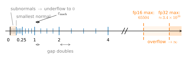
The exponent determines range, while the mantissa determines relative precision. Between adjacent powers of two, representable values are evenly spaced; the absolute spacing doubles at each power, and every format has a finite overflow threshold.
Machine epsilon \varepsilon_{\text{mach}} = 2^{-p} is the gap from 1 to its successor: \mathrm{fl}(x) = x(1+\delta), |\delta| \le \tfrac12 \varepsilon_{\text{mach}}.
fp8: E4M3 and E5M2
Floating point
Hardware also supports two fp8 formats. E4M3 has \varepsilon=0.125 and is commonly used for weights and activations. E5M2 gives up one mantissa bit for fp16’s exponent range and is often used for gradients:
float8_e4m3fn  eps = 0.125  smallest normal =     0.015625  max =   448.0
  float8_e5m2  eps =  0.25  smallest normal = 6.103515625e-05  max = 57344.0
Practical fp8 training uses explicit tensor- or block-level scale factors to keep values within the representable range.
Where the thresholds are
Floating point
Because e^x turns additive scale into multiplicative scale, finite thresholds matter: exponentiation overflows near x \approx 88.7 in fp32 and x \approx 11.1 in fp16.
1 + eps   != 1 : True
1 + eps/2 == 1 : True
gap between adjacent float32 values near 1    : 1.1920929e-07
gap between adjacent float32 values near 2^20 : 0.125
float16: exp(x) overflows for x > 11.09
float32: exp(x) overflows for x > 88.72
fp16 gradients below 6\times10^{-5} enter the subnormal range and lose precision; values below about 6\times10^{-8} round to zero. Updates of relative size below \varepsilon_{\text{mach}}/2 can round to no update at all. Both effects matter in mixed-precision training.
Two fp16 failure modes require different remedies
Floating point
A true gradient of 10^{-8} underflows to zero in an fp16 backward pass. Scaling the loss by 2^{14} keeps the intermediate gradient representable. An update of relative size 10^{-4} is lost when applied to an fp16 weight, but remains effective when applied to an fp32 master copy:
fp16 gradient, no scaling      : 0.0
fp16 gradient, loss scale 2^14 : 1.000e-08
fp16 step w - lr*g leaves w unchanged : True
fp32 master copy takes the step       : 0.999900
Loss scaling is underflow management; master weights are rounding management. This is precisely what torch.amp’s GradScaler plus fp32 master weights automate. Bfloat16’s fp32-sized exponent often removes the need for loss scaling, but not for stable exponentials or accurate accumulation.
02
Softmax & cross-entropy
overflow and a shift-invariant formulation
Softmax overflows; subtract the max
Stable softmax
Direct evaluation of \mathrm{softmax} exponentiates logits, so any logit past 88.7 makes the numerator inf and the ratio NaN. But softmax is shift-invariant:
\mathrm{softmax}(\mathbf{z} - c\mathbf{1}) = \mathrm{softmax}(\mathbf{z}),
so, for finite logits, shift by c = \max_i z_i: every exponent is \le 0, the denominator sits in [1,n], and exponential overflow is avoided.
naive,  logits z      : [0.09003058 0.24472846 0.66524094]
naive,  logits z + 100: [nan nan nan]
stable, logits z + 100: [0.09003057 0.24472846 0.66524094]
naive and stable agree where both work: False
Log-sum-exp: an exact, safe identity
Stable softmax
The same shift gives a stable expression for the softmax normalizer:
\mathrm{lse}(\mathbf{z}) = \log\textstyle\sum_j e^{z_j}
= c + \log\textstyle\sum_j e^{z_j - c},
\qquad \max_j z_j \le \mathrm{lse}(\mathbf{z}) \le \max_j z_j + \log n.
Direct exponentiation of logits near 1000 overflows even in float64, while the log-space expression remains finite:
naive  log(sum(exp(z))) : inf
stable log_sum_exp(z)   : 1002.4076
log softmax             : [-2.4075928  -1.4075928  -0.40759277]
probabilities sum to 1  : 1.000013
A soft maximum, within \log n of the true max, and the reason naive Bayes sums logs instead of multiplying probabilities.
Pass logits, not probabilities
Stable softmax
Cross-entropy can be computed directly from logits with one stable lse:
-\log\mathrm{softmax}(\mathbf{z})_y = \mathrm{lse}(\mathbf{z}) - z_y.
The via-probabilities route forces the loss through the representable range of probabilities and fails in one of three ways, depending on the library: subnormal noise before inf, inf outright, or a silent clip:
gap    CE from logits    CE via probabilities
   20          20.0000          20.0000
   60          60.0000          60.0000
  103         103.0000         103.2789
  104         104.0000              inf
How the from-probabilities route fails
Stable softmax
The label is the unlikely class, so the true loss is the logit gap. From logits it is exact at every gap; via probabilities it fails:
PyTorch. Matches until e^{-t} falls among the subnormals: at gap 103 the loss reads 103.2789 (wrong in the first decimal, no warning), and at gap 104 it underflows to inf.
Losses and likelihoods should remain in log space until probabilities are explicitly needed.
03
Catastrophic cancellation
subtracting near-equal numbers
Cancellation amplifies existing error
Cancellation
Subtracting nearby floating-point values can be exact, yet cancellation of their leading digits exposes errors already present in the operands. The relative-error amplification factor \tfrac{|a|+|b|}{|a-b|}u becomes large when a\approx b. In float32, 1+10^{-8} rounds to 1, so \log(1+x) returns zero, whereas log1p retains the increment:
float32 rounds 1 + x to     : 1.0
log(1 + x) = 0.0    log1p(x) = 1e-08
a - b in float32            : 2.3841858e-07   (true value 3.0e-07)
amplification (|a|+|b|)/|a-b| ~ 8.4e+06
Common examples include \log(1+x) and e^x-1 near zero (log1p and expm1), 1-\cos x, and the quadratic formula near a double root. Prefer a stable reformulation; higher precision alone does not remove the amplification.
Stable one-pass variance
Cancellation
The one-pass variance formula \mathbb{E}[x^2] - \mathbb{E}[x]^2 subtracts two numbers near \mu^2 to get \sigma^2, amplification \mu^2/\sigma^2. Welford keeps a running mean and centered sum of squares, so nothing large is ever subtracted:
m_k = m_{k-1} + \frac{x_k - m_{k-1}}{k},
\qquad M_k = M_{k-1} + (x_k - m_{k-1})(x_k - m_k).
Mean 10^9, true variance 1, 10^5 samples, all in float64:
naive E[x^2] - E[x]^2 :   384.000000
Welford, one pass     :     1.000257
two-pass reference    :     1.000257
The naive formula is off by a factor of several hundred in double precision; Welford agrees with the two-pass reference to eight digits. This is how BatchNorm tracks running moments.
Summation order is an algorithm
Cancellation
The direct variance calculation changes sign across NumPy builds because the summation order changes its rounding error. Left-to-right summation of n values performs one rounded addition per value and has worst-case error of order nu. More stable methods reorganize or compensate the additions:
left-to-right O(n\,u) · pairwise (sum halves recursively) O(u \log n) (what NumPy’s sum does, blocking and all) · Kahan (carry each rounding in a second accumulator) O(u), independent of n
Welford composes with either: the pairwise merge rule is exactly how running moments are combined across devices.
04
Conditioning
backward error, forward error, and κ
Backward and forward error
Conditioning
Forward error measures \|\hat{\mathbf{x}}-\mathbf{x}\|. Backward error measures the smallest input perturbation for which \hat{\mathbf{x}} is exact. The condition number relates the two:
\frac{\|\hat{\mathbf{x}} - \mathbf{x}\|}{\|\hat{\mathbf{x}}\|}
\le \kappa(\mathbf{A})\,\varepsilon.
correct digits \approx format digits -\,\log_{10}\kappa(\mathbf{A}). A backward-stable float64 solve begins with about 16 decimal digits, and a condition number \kappa=10^k can remove approximately k of them.
Hilbert matrices: the rule of thumb, verified
Conditioning
\kappa of the Hilbert matrix H_{ij} = 1/(i{+}j{-}1) grows exponentially. Solving \mathbf{H}\mathbf{x} = \mathbf{b} with \mathbf{x} = \mathbf{1}, the surviving digits track the rule of thumb row by row:
 n      kappa   log10 kappa   forward error  correct digits  backward error
 4    1.6e+04       4.2         4.1e-14         13.4         0.0e+00
 6    1.5e+07       7.2         1.4e-10          9.8         1.3e-16
 8    1.5e+10      10.2         6.1e-08          7.2         5.7e-17
10    1.6e+13      13.2         8.7e-05          4.1         1.0e-16
12    1.8e+16      16.2         3.2e-01          0.5         9.8e-17
The backward error remains near 10^{-16} in every row. The matrix’s conditioning, rather than the solver’s backward error, amplifies the error.
Normal equations square the condition number
Conditioning
Solving least squares via \mathbf{A}^\top\mathbf{A}\,\mathbf{w} =
\mathbf{A}^\top\mathbf{b} replaces \kappa(\mathbf{A}) with its square:
\kappa(\mathbf{A}^\top\mathbf{A}) = \kappa(\mathbf{A})^2.
With \kappa(\mathbf{A}) = 10^5, that is five extra digits lost versus an SVD/QR solve on \mathbf{A} directly:
kappa(A) = 1.0e+05   kappa(A^T A) = 1.0e+10
normal equations: relative error 7.7e-08  (7.1 correct digits)
SVD (lstsq)     : relative error 5.5e-14  (13.3 correct digits)
Numerical libraries commonly implement lstsq with QR or SVD so that they do not square the condition number by explicitly forming \mathbf{A}^\top\mathbf{A}.
Ridge regularization as preconditioning
Conditioning
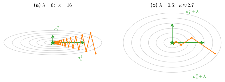
Adding \lambda\|\mathbf{w}\|^2 lifts every eigenvalue of \mathbf{A}^\top\mathbf{A} by \lambda, so \kappa = \tfrac{\sigma_1^2 + \lambda}{\sigma_n^2 + \lambda}\downarrow 1. This improves the accuracy of linear solves and the rate of gradient descent. Unlike a true preconditioner, ridge changes the minimizer: it shrinks \mathbf{w}_\lambda toward \mathbf{0}.
iterations / kappa: [5.89 5.9 5.94 5.99 6.06 6.15 6.19 6.25 6. ]
Stable algorithms control error; conditioning controls sensitivity
Wrap-up
- Floating point: relative precision \varepsilon_{\text{mach}}, gaps that double, overflow thresholds (e^x overflows at x\approx 88.7 in fp32).
- Stable softmax: subtract the max; log-sum-exp is exact; compute cross-entropy from logits as \mathrm{lse}(\mathbf{z}) - z_y.
- Cancellation: use stable reformulations such as
log1p and Welford’s recursion.
- Conditioning: forward error is bounded by \kappa times backward error; normal equations square \kappa, while ridge regularization reduces it.
The condition number affects both the accuracy of a linear solve and the convergence rate of fixed-step gradient descent. Ridge regularization reduces it in both settings, while also changing the statistical objective.