Proof. Insert \pm\mathbf m(X); the cross term vanishes by the tower rule. \blacksquare Least squares against a noisy target fits its conditional mean: used once for scores, once for velocities.
Denoising score matching & Tweedie
Denoising
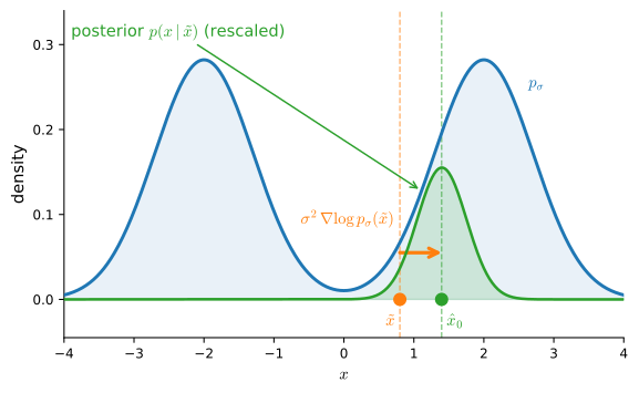
Perturb \tilde{\mathbf x}=\mathbf x+\sigma\boldsymbol\epsilon; the conditional score is closed-form -\boldsymbol\epsilon/\sigma, and regressing on it (Vincent) recovers the marginal score. Rearranged, that is Tweedie:
For Gaussian corruption and squared error, the score determines the posterior-mean denoiser through Tweedie’s formula.
A score network in 1-D
Denoising
A tiny MLP trained by denoising score matching approximates the analytic score, with loss close to a finite-sample estimate of the Bayes risk:
DSM loss 2.036 vs estimated Bayes risk 2.038; max |s_theta - score| on [-4, 4]: 0.199
02
Score-based diffusion
forward noise, DDPM, Langevin, DDIM, guidance
A noise schedule connects coverage to detail
Forward process
Small \sigma approximates p but provides little coverage of low-density regions; large \sigma provides coverage but over-smooths. Train a noise-conditional score \mathbf s_\theta(\mathbf x,t) trained along a forward SDE (VE or VP), then a reverse pass to generate:
A weighting \lambda(t) allocates effort across noise levels. Under the regularity and terminal-distribution assumptions of the cited analysis, \lambda=g^2 relates the population loss to an upper bound on negative log-likelihood; DDPM uses 1-\bar\alpha_t.
Two clocks
Conventions
Diffusion runs data→noise and samples backward; flow matching runs noise→data and samples forward. To compare, substitute t\to 1-t:
DDPM is a first-order VP discretization with exact marginals
DDPM
The DDPM step is Euler–Maruyama on the VP-SDE (to O(\beta_t)).
The simple \|\boldsymbol\epsilon-\boldsymbol\epsilon_\theta\|^2 loss is denoising score matching, reweighted by \lambda(t)=1-\bar\alpha_t.
t =   10: Var(x_t) chain 1.000, formula 1.000, alpha_bar 0.9981
t =  100: Var(x_t) chain 0.994, formula 1.000, alpha_bar 0.8970
t = 1000: Var(x_t) chain 1.024, formula 1.000, alpha_bar 0.0000
chain vs one-shot at T: mean -0.027 vs +0.005, std 1.012 vs 1.000
Langevin: stationary but slow
Sampling
dX = \tfrac12\nabla\log p\,dt + dW has stationary density p (substitute \rho=p into Fokker–Planck → 0). But it mixes slowly across modes:
From one mode, almost no chain crosses (P(X>0)=0.012). Annealed noise or a predictor–corrector method improves movement between modes.
DDIM: deterministic updates from conditional estimates
Sampling
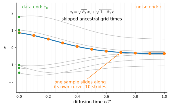
Invert the marginal for \hat{\mathbf x}_0 = \bigl(\mathbf x_t - \sqrt{1-\bar\alpha_t}\,\boldsymbol\epsilon_\theta\bigr)/\sqrt{\bar\alpha_t}, then re-use the predicted noise instead of resampling:
The update is deterministic and can skip levels. Its predicted noise is a conditional mean, not the latent noise realization of an individual forward sample, so a finite stride is approximate.
Sparse DDIM strides trade evaluations for bias
Sampling
On the closed-form mixture, with no learned approximation, ten strides place every sample in the same mode as the thousand-step numerical reference; at fifty strides the paired empirical CDF gap is 0.018:
 10 strides vs 1000: mean |gap| 0.083, KS 0.080, mode fraction 0.495
 50 strides vs 1000: mean |gap| 0.015, KS 0.018, mode fraction 0.495
mode fraction at 1000 steps: 0.495; the same initial draws are used at every stride count
Same network; \eta controls reinjected noise. In the fine-step limit, deterministic DDIM is related to the probability-flow ODE; finite strides are numerical approximations, including for Gaussian marginals.
Classifier-free guidance trains one network with label dropout and extrapolates through the conditional: \tilde{\mathbf s} = (1-\gamma)\,\mathbf s_\varnothing + \gamma\,\mathbf s_y.
Measured on the closed-form mixture: \gamma=1 closely approximates the exact conditional (mean 0.966 vs the analytic 0.970); at \gamma=3, 10 there is no additional mass to reallocate, so the mode shifts to 1.04, then 1.07, and narrows.
For \gamma>1 the tilt p_t(\mathbf x)\,p_t(y\mid\mathbf x)^\gamma is not, in general, the noised marginal of a clean distribution: it is a controlled distortion rather than a consistent diffusion path.
03
Flow matching
prescribe the path, regress the velocity, translate the targets
Probability paths and velocities
Flow matching
Prescribe a path (p_t) from noise to data; its velocity obeys the continuity equation. The intractable marginal velocity is again a posterior mean:
The same conditional-expectation argument used for score matching applies.
The conditional flow-matching theorem
Flow matching
Under the theorem’s integrability assumptions, the population CFM loss (closed-form per-pair velocity) and the population FM loss have the same gradients.
Proof. Apply the regression lemma with target \mathbf u_t(\mathbf x\mid\mathbf z); its conditional mean is the marginal velocity. \blacksquare Identical structure to Vincent’s theorem.
Relations among score, noise, and velocity
Parameterization relations
On a Gaussian path, at times where \alpha_t,\sigma_t>0, \mathbf x_t = \alpha_t\,\mathbf x_1 + \sigma_t\,\boldsymbol\epsilon, the marginal velocity and the marginal score determine each other:
sampled components remain comparable under common normalized schedules
The log-SNR coordinate \rho_t=\log(\alpha_t^2/\sigma_t^2) compares schedules. After state rescaling, matching \rho ranges can describe the same noised marginals up to time reparameterization; velocity scaling and numerical cost still change with the clock.
Rectified flow: straight paths
Flow matching
The simplest path is a straight line, \mathbf x_t=(1-t)\mathbf x_0+t\mathbf x_1, with constant target \mathbf x_1-\mathbf x_0. Conditional paths are straight; the marginal flow curves where conditional paths intersect:
Euler step count resolves the learned two-moons geometry
Flow matching
A small MLP trained by the rectified-flow loss is integrated with Euler’s method. The generated crescents become more accurate as the step count grows:
One reflow round reduces one-step error in this run
Reflow
Integrate the trained ODE once, keep the model-generated couplings (\mathbf z, \hat{\mathbf x}_1(\mathbf z)), and retrain the same architecture on those pairs:
final reflow loss 0.001
 1 step(s): energy distance  CFM 0.676  ->  reflow 0.016
 2 step(s): energy distance  CFM 0.163  ->  reflow 0.015
32 step(s): energy distance  CFM 0.014  ->  reflow 0.016
In this two-moons run, one Euler step scores 0.016, close to the original model’s 32-step score of 0.014 and better than its one-step 0.676. The smaller loss is consistent with a much smaller posterior variance under the new coupling; it is not a zero-variance guarantee for finite training.
For distributions with finite second moments and admissible regular flows, any bridging flow costs at least W_2^2 (Jensen); a minimizing displacement interpolation moves particles in straight lines at constant speed.
Benamou–Brenier identifies kinetic energy exactly. Curvature can increase low-order truncation error, but solver cost also depends on derivatives, conditioning, tolerances, and the method. Reflow and OT couplings aim to reduce these costs; neither certifies them for a finite learned field.
Step count and solver order control distinct errors
Sampling
For the learned two-moons field, the sample metric decreases with Euler step count and then plateaus; the plateau does not by itself identify model error separately from finite-sample variability:
steps_list = [1, 2, 4, 8, 16, 32, 64]eds = [energy_distance(euler_sample(2048, K), held_out) for K in steps_list]print(' '.join(f'{K}: {e:.3f}'for K, e inzip(steps_list, eds)))d2l.plot(steps_list, eds, 'Euler steps', 'squared energy distance', xscale='log', yscale='log')
For the analytic one-dimensional field below, Heun at 20 steps (40 field evaluations) beats Euler at 40 steps relative to the fine numerical reference, as the observed second-order convergence predicts:
Conditional regression supplies several learned dynamics
Sampling
These methods share three components: a probability path, a closed-form conditional regression target, and a numerical integrator.
DDPM, score-SDE, PF-ODE, DDIM, and flow matching can be compared by path, target parameterization, loss weighting, and integrator. Stochastic interpolants provide one formalism for many, but not every implementation detail, in this family.
Recap
Wrap-up
The score is independent of Z; DSM (Vincent) regresses on -\boldsymbol\epsilon/\sigma; Tweedie’s formula gives the optimal denoiser.
Langevin mixes slowly; DDIM is deterministic; guidance is Bayes on scores.
Flow matching prescribes the path; CFM = FM by the same regression lemma.
Score, noise, \hat{\mathbf x}_1, velocity: one posterior mean in different parameterizations, on the log-SNR clock.
Benamou–Brenier identifies the least-energy flow; on the two-moons run, one reflow round made one Euler step approach the original model’s 32-step metric.
Both DSM and CFM replace an intractable marginal field by regression on a tractable conditional target whose conditional mean is that field.