Generative Adversarial Networks

Dive into Deep Learning · §16.1

Generative adversarial networks
a sampler without a density · the log-loss game · the value is Jensen–Shannon · two generator weights

A High Likelihood Does Not Certify Good Samples

An implicit generator x' = G(z), z \sim \mathcal{N}(0, I): sampling is a forward pass, but the density of x' is unavailable, so maximum likelihood cannot apply.

And likelihood would be the wrong yardstick anyway:

\tilde p = 0.01\, p_{\textrm{data}} + 0.99\, p_{\textrm{noise}} \;\;\Rightarrow\;\; \log \tilde p(x) \geq \log p_{\textrm{data}}(x) - \log 100

  • Within 4.6 nats of optimal, against log-likelihoods in the thousands.
  • Yet 99% of its samples are noise. Likelihood therefore need not measure sample quality.

Two Networks, One Classification Problem

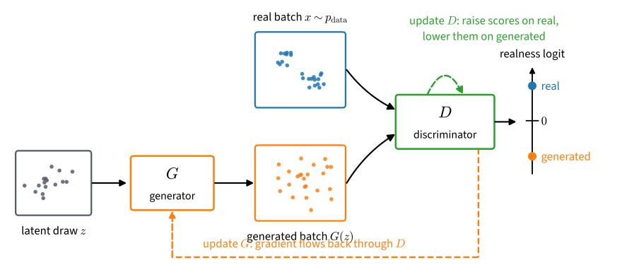
The discriminator maximizes, the generator minimizes:

V(D) = E_{x \sim p}[\log \sigma(D(x))] + E_{x' \sim q}[\log \sigma(-D(x'))]

Maximizing V = fitting the Bayes classifier of real vs. generated.

The Optimal Critic Is the Log Density Ratio

The supremum decouples across points: at each x, maximize p \log s + q \log(1-s) over s = \sigma(D(x)).

\sigma(D^\star) = \frac{p}{p+q}, \qquad D^\star = \log\frac{p}{q} = \lambda

  • The trained critic is a density-ratio estimator: it recovers the one function of q the game needs, though q itself has no formula.
  • The constant is pinned too: shifting D^\star strictly lowers V.

The Value of the Game Is Jensen–Shannon

\max_D V(D) = 2\,\mathrm{JS}(p, q) - 2\log 2, \qquad \mathrm{JS}(p,q) = H[m] - \tfrac{1}{2}(H[p] + H[q])

  • Entropy reading: the uncertainty the unknown origin adds to a sample.
  • Information reading: \mathrm{JS}(p,q) = I(x; y), the nats one sample carries about which distribution produced it.
  • Hence 0 \leq \mathrm{JS} \leq \log 2: the ceiling is reached on disjoint supports, where every sample identifies its source.

Two Generator Losses, Two Sample Weights

Both generator losses push samples up the critic’s score surface; they differ in the per-sample weight:

w_{\textrm{sat}}(x') = \sigma(D(x')), \qquad w_{\textrm{ns}}(x') = \sigma(-D(x'))

  • The saturating weight is near zero for confidently rejected samples, so those samples contribute little to the update.
  • The non-saturating weight is near one for the same samples.
  • With an optimal critic, both losses have the same fixed point q = p.

A Gaussian Test with Analytic Reference Values

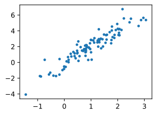
Data = z A + b: a Gaussian with known mean and covariance. A linear generator keeps q Gaussian too, so \log(p/q) and \mathrm{KL}(q\|p) have closed forms to check against.

torch.manual_seed(0)
Z = torch.normal(0.0, 1.0, (1000, 2))
A = torch.tensor([[1.0, 2.0], [-0.1, 0.5]])
b = torch.tensor([1.0, 2.0])
data = Z @ A + b
d2l.set_figsize()
d2l.plt.scatter(data[:100, 0], data[:100, 1], s=8);
print(f'covariance of the data distribution:\n{A.T @ A}')

covariance of the data distribution:
tensor([[1.0100, 1.9500],
        [1.9500, 4.2500]])

The Value Appears in the Loss Curves

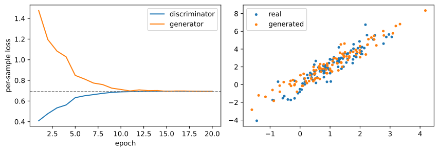
At the end of training, both per-sample losses sit at \log 2 \approx 0.693. For a discriminator near its best response, this value is consistent with \mathrm{JS} \approx 0; the generated cloud provides a separate visual check.

The Trained Critic Tracks the Analytic Log Ratio

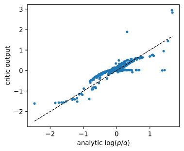
Freeze a partially trained generator; train the critic to its best response; compare with the closed-form \lambda = \log(p/q):

correlation(D, lambda) = 0.868
mean |D - lambda| = 0.157 nats
Text(0, 0.5, 'critic output')

Points hug the identity line; errors grow only where the mixture has almost no samples, because ratio estimation is unconstrained off-support.

Saturation under an Identical Initialization

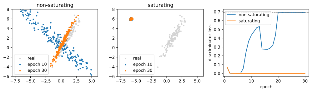
Start the generator far from the data, where the critic rejects confidently; train the same initialization under each weighting:

The non-saturating run moves toward the data. The saturating run remains near its initialization because \sigma(D(x')) \approx 0 for every generated sample.

Recap

  • An implicit generator has no tractable density, and likelihood need not reflect sample quality. A learned comparison provides a training signal.
  • Optimal critic: \sigma(D^\star) = p/(p+q), logit = \log(p/q): a density-ratio estimator.
  • Value of the game: 2\,\mathrm{JS}(p,q) - 2\log 2; \mathrm{JS} = I(x;y) \leq \log 2.
  • Generator weights: \sigma(D) vanishes on confidently rejected samples, whereas \sigma(-D) remains near one; both have the same fixed point.
  • In the Gaussian experiment, losses approach \log 2, the critic approximates \lambda, and KL falls from roughly eight nats to a fraction of a nat.
  • Disjoint supports still fix the objective at \log 2 and remove the gradient. The next section addresses this limitation.