Deep Q-Networks

Dive into Deep Learning · §15.4

Deep Q-Networks
instability under function approximation · experience replay and target networks · termination and truncation · maximization bias and Double DQN

Sources of Instability

Unlike the policy-gradient target, the Q-learning target depends on the function being trained:

y = r + \gamma\, \big(1 - \mathbf{1}(s' \textrm{ terminal})\big) \max_{a'} Q_w(s', a')

  • The tabular convergence argument, based on stochastic approximation to a contraction, no longer applies after projection onto a function class :cite:Tsitsiklis.VanRoy.1997.
  • Consecutive transitions are strongly correlated, and each parameter update changes the estimates for many states.
  • Replay decorrelates the data but makes them off-policy, so the critic is no longer trained solely on the current policy’s state distribution.

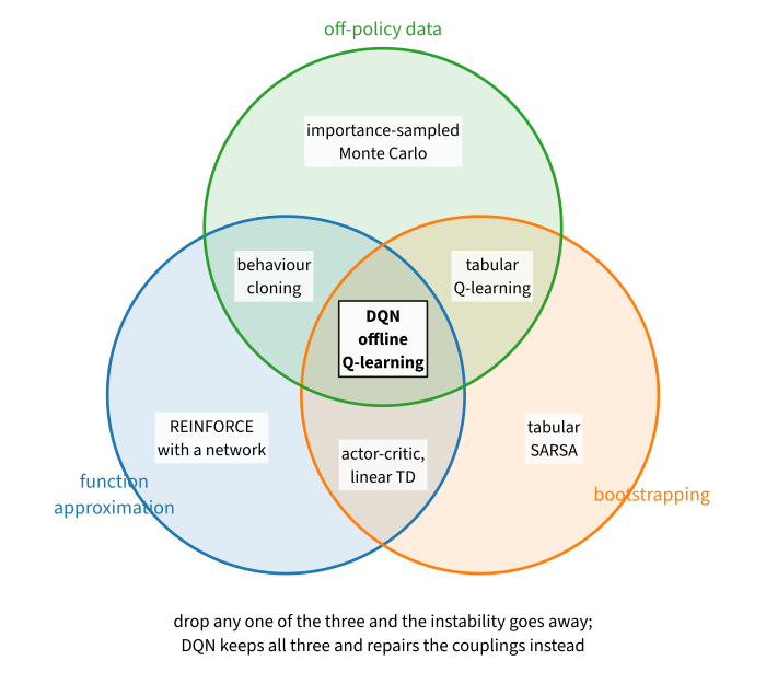
The Deadly Triad

Function approximation + bootstrapping + off-policy data :cite:Sutton.Barto.2018,vanHasselt.Doron.Strub.ea.2018. Every region is an algorithm already taught:
Baird’s Counterexample

Baird’s construction has seven states and zero true value everywhere, which the parameterization can represent with w=0. Even deterministic expected updates diverge under uniform off-policy weighting:
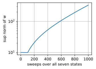
sup norm of w after 0, 500, 1000 sweeps: 10, 77, 335
the value the weights claim for state 7: 677, true value 0

The parameters diverge exponentially for every positive constant step size. The failure belongs to the expected update operator, not to sampling noise :cite:Baird.1995.

Replay and Target Networks
Experience Replay and Off-Policy Data

class ReplayBuffer:
    """A ring of transitions in preallocated numpy; sample() returns a Batch."""
    def __init__(self, capacity, obs_dim):
        self.obs = np.zeros((capacity, obs_dim), np.float32)
        self.act = np.zeros(capacity, np.int64)
        self.rew = np.zeros(capacity, np.float32)
        self.next_obs = np.zeros((capacity, obs_dim), np.float32)
        self.term = np.zeros(capacity, np.float32)
        self.capacity, self.size, self.ptr = capacity, 0, 0

    def add(self, obs, act, rew, next_obs, term):
        i = self.ptr
        self.obs[i], self.act[i], self.rew[i] = obs, act, rew
        self.next_obs[i], self.term[i] = next_obs, term
        self.ptr, self.size = (i + 1) % self.capacity, min(self.size + 1,
                                                           self.capacity)

    def __len__(self):
        return self.size

    def sample(self, batch_size, rng):
        i = rng.integers(self.size, size=batch_size)
        return d2l.Batch(self.obs[i], self.act[i], self.rew[i],
                         self.next_obs[i], self.term[i],
                         np.array([batch_size]))
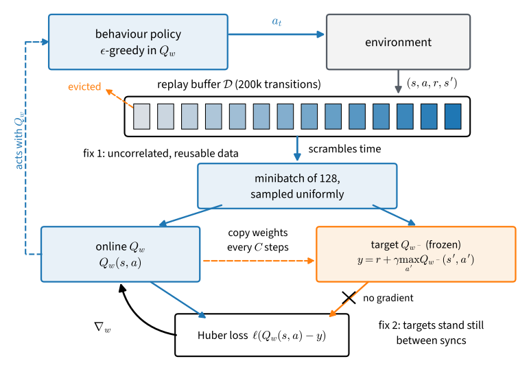
  • The Q-learning target does not depend on the behavior policy, so transitions collected by other policies remain usable (:numref:sec_qlearning).
  • A sampled Batch no longer preserves episode order. Consequently, reward_to_go and gae cannot be computed from it, while the one-step td_target remains available.
  • The replay capacity is 200,000 transitions and the experiment uses only 50,000 environment steps, so no transition is evicted.

The Target Network

y = r + \gamma\, \big(1 - \mathbf{1}(s' \textrm{ terminal})\big) \max_{a'} Q_{w^-}(s', a'), \qquad w^- \leftarrow w \textrm{ every } C \textrm{ steps}

Between synchronizations, the regression target is fixed.

The actor–critic method in :numref:sec_actorcritic recomputed its bootstrap target on every pass using fresh on-policy data. DQN instead freezes a copy of the value network to reduce feedback between an update and its target. The use_target=False ablation synchronizes this copy after every step and is therefore equivalent to using the online network in the target.

The Training Loop

def train_dqn(seed, qnet, use_target=True, step=None):
    """DQN on CartPole; yields (env step, episode return, max_a Q(s0, a))."""
    step = q_step if step is None else step
    rng, env = np.random.default_rng(seed), gym.make('CartPole-v1')
    target = make_qnet()
    target.load_state_dict(qnet.state_dict())
    opt = torch.optim.Adam(qnet.parameters(), lr=lr)
    buffer, s0 = ReplayBuffer(buffer_size, 4), np.zeros(4, np.float32)
    obs, ep_return = env.reset(seed=seed)[0], 0.0
    sync = sync_every if use_target else 1
    for t in range(1, num_env_steps + 1):
        a = d2l.epsilon_greedy(q_values(qnet, obs), epsilon(t), rng)
        next_obs, rew, terminated, truncated, _ = env.step(a)
        buffer.add(obs, a, rew, next_obs, float(terminated))
        obs, ep_return = next_obs, ep_return + rew
        if terminated or truncated:
            yield t, ep_return, q_values(qnet, s0).max()
            obs, ep_return = env.reset()[0], 0.0
        if len(buffer) >= warmup and t % train_freq == 0:
            step(qnet, target, opt, buffer.sample(batch_size, rng))
        if t % sync == 0:
            target.load_state_dict(qnet.state_dict())

The budget is 50,000 environment steps, with one gradient update after every two steps. The implementation reuses epsilon_greedy and linear_schedule from :numref:sec_qlearning. The replay buffer records terminated rather than truncated so that a time limit does not suppress bootstrapping.

Target-Network Ablation

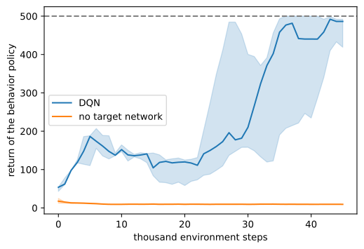
With a target network, every seed reaches returns in the hundreds, although performance remains variable. Without it, every seed in both implementations falls to near-minimal return and its value estimates exceed 10^8. In this ablation, removing the target network therefore causes clear divergence.

Value-Loss Diagnostics

               DQN: best 20-episode window per seed [500. 348. 457.]
                    final window [496. 348. 431.] (spread 148)
                    fifty episodes earlier [163.  99. 203.]
 no target network: best 20-episode window per seed [30. 27. 25.]
                    final window [9. 9. 9.] (spread 0)
                    fifty episodes earlier [10. 10. 10.]

Because performance rises and falls during training, the final moving average varies by more than one hundred points across seeds and changes if evaluated 50 episodes earlier. Reporting the best window would introduce post-selection bias. We therefore use a greedy evaluation at the fixed training budget as the primary result.

Converging Values, Churning Policy

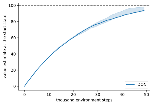
continuing-task ceiling: 100; the no-target arm ends at 1e+08, 1e+08, 1e+08

At the probe state, the value estimate approaches the correct scale rather than diverging; a single probe, however, cannot certify the whole value function. Small changes in action values can still change the greedy policy, and fixed-budget evaluations range from 90 to 500 across seeds and implementations. Because the update bootstraps through the time limit, it optimizes a continuing objective whose start-state value is bounded by 1/(1-\gamma)=100. Estimates above this bound are necessarily overestimates.

Maximization Bias

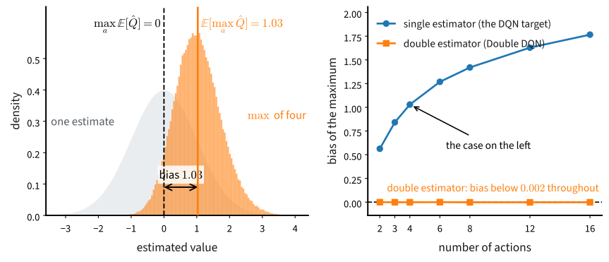
single estimator, E[max of the estimates]: 1.031
select with one, evaluate with the other: -0.006

In this example, applying \max to noisy estimates introduces approximately one unit of positive bias :cite:Thrun.Schwartz.1993. Using independent estimates for selection and evaluation removes the bias :cite:vanHasselt.2010. The hard maximum is the \beta\to0 limit of the soft backup in :numref:sec_regularized.
The Double DQN Target

Select with the online network, evaluate with the frozen one :cite:Hasselt.Guez.Silver.2016:

def q_step_double(qnet, target, opt, batch):
    """q_step with selection split from evaluation, eq_double_dqn."""
    sel = q_values(qnet, batch.next_obs).argmax(-1)
    fit_q(qnet, opt, batch, batch.td_target(
        lambda s: q_values(target, s)[np.arange(len(s)), sel], gamma))
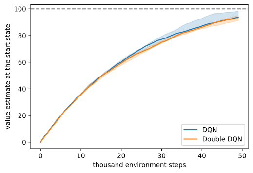
       DQN: final value estimate at s0, per seed: [93.8 98.3 93. ]
Double DQN: final value estimate at s0, per seed: [92.6 95.1 91. ]

Most seeds finish with values a few points lower under Double DQN. This small difference is consistent with the two-action experiment in panel (b), where maximization has limited scope to select extreme errors. On Atari, with as many as 18 actions, the same modification produces substantially larger effects.

DQN in Modern Practice

  • n-step targets extend the return construction developed in :numref:sec_actorcritic.
  • Prioritized replay :cite:Schaul.Quan.Antonoglou.ea.2016, dueling networks :cite:Wang.Schaul.Hessel.ea.2016, and distributional value heads :cite:Bellemare.Dabney.Munos.2017 are combined and ablated in Rainbow :cite:Hessel.Modayil.vanHasselt.ea.2018.
  • PQN :cite:Gallici.Fellows.Ellis.ea.2025 uses LayerNorm and parallel environments without a replay buffer or target network, illustrating that replay and target networks are not the only route to stable value learning.
  • Modern applications often use PPO or newer value-based agents. DQN remains a useful setting in which to study the principal failure modes. :numref:sec_offline next considers the limiting case of fully offline data.