Actor-Critic Methods and Multi-Step Returns

Dive into Deep Learning · §15.1

Actor-critic and the credit-assignment dial
bootstrapped advantage estimates · coupled actor and critic updates · generalized advantage estimation · measured bias and variance

Bootstrapping the Reward-to-Go

The Monte Carlo weight waits for the episode to end. But \hat G_t = r_t + \gamma \hat G_{t+1}, and \hat V(s_{t+1}) is trained to predict exactly what \hat G_{t+1} samples. Substitute:

\delta_t = r_t + \gamma\, \hat V(s_{t+1}) - \hat V(s_t)

:eqref:eq_td_error’s scalar, with the max replaced by the policy’s own continuation.

@d2l.add_to_class(d2l.Batch)
def td_target(self, bootstrap, gamma):
    """r_t + gamma (1 - terminated) V(s'), by a numpy bootstrap."""
    return self.rew + gamma * (1 - self.term) * bootstrap(self.next_obs)

Because a NumPy array carries no gradient graph, the target is treated as data by construction. No explicit detach operation is needed.

Why the TD Error Is an Advantage

If the critic were exact, \hat V = V^\pi:

E[\delta_t \mid s_t, a_t] = Q^\pi(s_t, a_t) - V^\pi(s_t).

A single transition therefore provides an advantage estimate, whereas the Monte Carlo estimate requires the rest of the trajectory.

During training, however, \hat V generally differs from V^\pi, so this estimate is biased. Actor–critic methods accept this bias in exchange for lower variance.

Actor and Critic Updates

w \leftarrow w + \alpha_w\, \delta_t\, \nabla_w \hat V_w(s_t), \qquad \theta \leftarrow \theta + \alpha_\theta\, \delta_t\, \nabla_\theta \log \pi_\theta(a_t \mid s_t)

• The critic performs sampled, bootstrapped policy evaluation. Actor–critic is therefore an instance of generalized policy iteration in which both evaluation and improvement are approximate.
• A two-timescale heuristic lets the critic learn faster than the actor because its target changes with both networks. Here we take 20 fitted-TD passes, recomputing the target on each pass, before updating the actor.

A Batched Actor-Critic

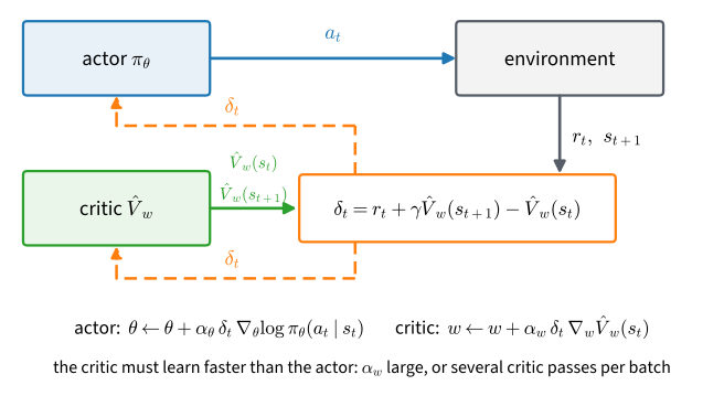
The following implementation collects a batch of episodes and takes one actor step per batch. It is a single-environment teaching analogue of A2C :cite:Mnih.Badia.Mirza.ea.2016. Relative to the loop in :numref:sec_deeprl, only the final update changes:

def train_ac(seed, ac, num_updates=num_updates):
    """The same loop with the sampled tail replaced by the bootstrap."""
    rng, env = np.random.default_rng(seed), gym.make('CartPole-v1')
    env.reset(seed=seed)
    for _ in range(num_updates):
        batch = d2l.rollout(env, ac.act, batch_episodes, rng)
        for _ in range(critic_steps):   # fresh target, one pass, repeat
            fit_value(ac, batch.obs, batch.td_target(ac.value_np, gamma))
        delta = batch.td_target(ac.value_np, gamma) - ac.value_np(batch.obs)
        gnorm = policy_step_clip(ac, batch, d2l.normalize(delta))
        yield float(batch.episode_returns().mean()), gnorm

The critic uses td_target instead of G, takes critic_steps passes before the actor update, and supplies the normalized TD error \delta_t as the actor’s weight.

CartPole, Three Seeds Each

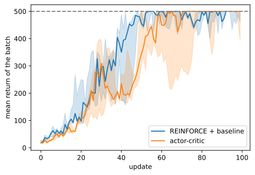
Actor–critic learns more slowly at first while its critic is inaccurate. Later, both methods reach the 500-step ceiling, but only actor–critic remains there for long consecutive intervals in these runs.

Return and Stability

REINFORCE + baseline: longest stretch of perfect batches, per seed: [6, 7, 4]
        actor-critic: longest stretch of perfect batches, per seed: [36, 26, 11]

A perfect batch contains eight episodes of length 500. Only actor–critic produces long sequences of such batches in these runs. This observation is consistent with the greater sampling variance of Monte Carlo returns, though three seeds do not establish a general stability result.

Gradient-Norm Comparison

REINFORCE + baseline: median pre-clip gradient norm  0.04, clip binds on   0% of updates
        actor-critic: median pre-clip gradient norm  0.40, clip binds on  35% of updates

Although both weights are normalized to unit variance, the actor–critic gradient norms are an order of magnitude larger in this experiment. A state-dependent component of the weight contributes variance but cancels in expectation, as shown in :numref:sec_baselines. The result is therefore consistent with the TD error concentrating more of its variation in action-dependent signal. :numref:sec_ppo develops a more accurate advantage estimator.

Critic Targets and Fresh Data

Rerun the loop, measuring both candidate weights per batch:

• The identity \hat G_t - \hat V(s_t) = \delta_t + \gamma(\hat G_{t+1} - \hat V(s_{t+1})) separates the shared one-step term from the remaining trajectory.
• Their correlation falls from about 0.3 toward zero as episodes approach 500 steps. This is a descriptive diagnostic, not evidence that the critic is accurate.
• The variance of the Monte Carlo weight grows with the horizon, whereas the TD-error variance remains nearly constant; their median ratio eventually exceeds one hundred.

Fresh on-policy data keeps the critic’s training distribution close to the current policy’s state distribution, reducing one source of mismatch. This is not a convergence guarantee: nonlinear TD can diverge even on-policy :cite:Tsitsiklis.VanRoy.1997. Our critic recomputes its target on every fitted-TD pass. In the off-policy setting of :numref:sec_dqn, a frozen target network is used instead.

The Multi-Step Return Parameter

\hat G^{(n)}_t = r_t + \cdots + \gamma^{n-1} r_{t+n-1} + \gamma^n \hat V(s_{t+n}), \qquad \hat A^{\textrm{GAE}}_t = (1-\lambda) \sum_{n \ge 1} \lambda^{n-1} \big(\hat G^{(n)}_t - \hat V(s_t)\big)

Telescoping identity :cite:Schulman.Moritz.Levine.ea.2016:

\hat A^{\textrm{GAE}}_t = \sum_{l \ge 0} (\gamma\lambda)^l\, \delta_{t+l}

Expanding each n-step return into TD errors and exchanging the sums leaves the geometric coefficient \lambda^l. TD(\lambda) computes the analogous quantity online with eligibility traces, an approach that remains useful in streaming settings :cite:Elsayed.Vasan.Mahmood.2024.

Computing GAE by a Backward Scan

@d2l.add_to_class(d2l.Batch)
def gae(self, value_fn, gamma, lam):
    """GAE(gamma, lam): the reward-to-go scan, run on the TD errors."""
    delta = self.td_target(value_fn, gamma) - value_fn(self.obs)
    return self.backward_scan(delta, gamma * lam)

The same backward scan used for reward-to-go in :numref:sec_baselines can be applied to TD errors.

lambda = 0 is the TD error; lambda = 1 is the Monte Carlo advantage

The tests verify both endpoint identities.

Comparing GAE Parameters

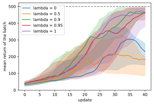
lambda =  0.0: best 20-update window, median 222.5, seeds [138. 198. 223. 283. 328.]
lambda =  0.5: best 20-update window, median 203.3, seeds [175. 179. 203. 218. 321.]
lambda =  0.9: best 20-update window, median 419.5, seeds [387. 400. 420. 454. 486.]
lambda = 0.95: best 20-update window, median 406.9, seeds [327. 367. 407. 444. 482.]
lambda =  1.0: best 20-update window, median 449.7, seeds [293. 385. 450. 464. 479.]

With five seeds per value of \lambda and 50 updates on small batches, low values of \lambda learn substantially more slowly. Values from 0.9 to 1 perform similarly. Because the critic is initially inaccurate, this short experiment favors estimators that rely more heavily on Monte Carlo returns.

Bias and Variance

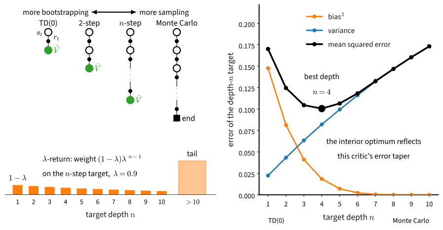
lambda =  0.0: relative bias 1.05, relative variance    0.1, one-draw error    1.2
lambda =  0.5: relative bias 1.06, relative variance    0.1, one-draw error    1.2
lambda =  0.9: relative bias 0.95, relative variance    0.2, one-draw error    1.1
lambda = 0.95: relative bias 0.83, relative variance    0.3, one-draw error    0.9
lambda =  1.0: relative bias 0.00, relative variance    1.6, one-draw error    1.6

The mean-squared error is shallow and U-shaped. As \lambda decreases from one, variance initially falls faster than squared bias grows; for still smaller values, bias dominates. The minimum therefore occurs between the two endpoints. PPO implementations commonly use \lambda between 0.9 and 0.97 (:numref:sec_ppo).

Recap

• The TD error is a one-transition advantage estimate. It is unbiased when \hat V = V^\pi and otherwise trades variance for bias.
• The critic performs sampled policy evaluation, so actor–critic is generalized policy iteration with approximate evaluation and improvement.
• In the batched implementation, the critic is updated before the actor.
• n-step returns and \lambda-returns interpolate between one-step TD and Monte Carlo returns; GAE computes the mixture with a backward scan.
• :numref:sec_ppo reuses each batch while controlling the policy update, and :numref:sec_dqn addresses off-policy learning with replayed data.