attention_weights = torch.eye(10).reshape((1, 1, 10, 10))
d2l.show_heatmaps(attention_weights, xlabel='Keys', ylabel='Queries')Attention as differentiable lookup
Over a database \mathcal{D} = \{(\mathbf{k}_1, \mathbf{v}_1), \ldots, (\mathbf{k}_m, \mathbf{v}_m)\}:
\textrm{Attention}(\mathbf{q}, \mathcal{D}) = \sum_{i=1}^m \alpha(\mathbf{q}, \mathbf{k}_i)\, \mathbf{v}_i.
One-hot \alpha gives exact lookup; uniform \alpha gives average pooling; other distributions interpolate between them.
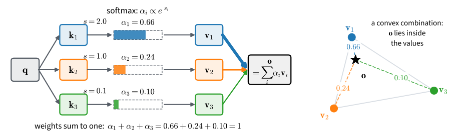
Attention pooling: a linear combination of values, with weights from query–key compatibility.
Visualizing attention weights
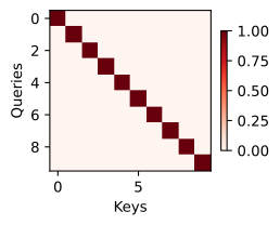
A queries-by-keys heatmap displays the weights. The identity matrix below represents exact lookup:
A 1964 attention mechanism
Nadaraya–Watson regression is attention pooling with a hand-picked similarity kernel:
f(\mathbf{q}) = \sum_i \mathbf{v}_i \frac{\alpha(\mathbf{q}, \mathbf{k}_i)}{\sum_j \alpha(\mathbf{q}, \mathbf{k}_j)}.
Keys = training inputs, values = labels, query = where to predict. The estimator requires no parameter training and is consistent if the kernel narrows at a suitable rate as data accumulate.
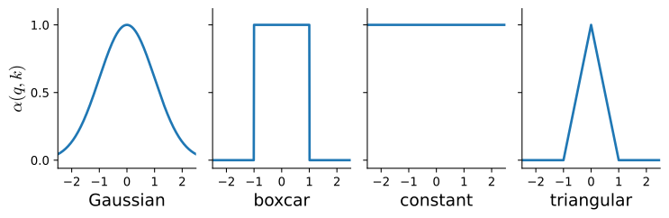
Gaussian, boxcar, constant, and triangular kernels.
Nadaraya–Watson in action
y = 2\sin(x) + x + \epsilon, 40 noisy points. Four lines of code: distances → kernel → normalize over keys → weighted sum of labels.
def nadaraya_watson(x_train, y_train, x_val, sigma):
    dists = x_train[:, None] - x_val[None, :]
    k = torch.exp(-dists**2 / (2 * sigma**2))
    attention_w = k / k.sum(0)  # Normalize over keys for each query
    return y_train @ attention_w, attention_w

sigmas = (0.1, 0.5, 2.0)
estimates = [nadaraya_watson(x_train, y_train, x_val, s)[0] for s in sigmas]
d2l.plot(x_val, estimates + [y_val], 'x', 'y',
         legend=[f'sigma = {s:g}' for s in sigmas] + ['truth'])
d2l.plt.plot(x_train, y_train, 'o', alpha=0.4);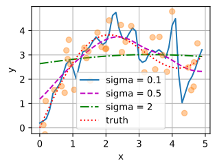
- In this example, the bandwidth \sigma has more effect than the choice among the displayed kernel shapes.
The weights explain the fits
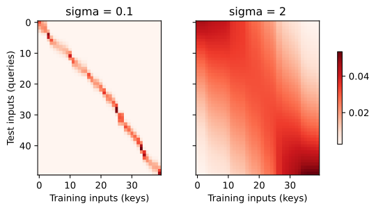
- Narrow kernel: sharp, local, noisy — weight on a handful of keys.
- Wide kernel: smooth, global — weight spread across the dataset.
- Either way the kernel is chosen, not learned, and every query gets the same notion of similarity.