Numerical Stability and Initialization
Dive into Deep Learning · §4.4
Numerical Stability and Initialization
Vanishing gradients, exploding gradients, and variance-preserving scales
Why does the starting point matter so much?
Motivation
A deep network composes many layers. Its initial weights strongly affect the scale of forward activations and backward gradients.
Three ideas made deep training routine:
- Non-saturating activations (ReLU).
- Variance-preserving init (Xavier, He).
- Symmetry breaking (different initial weights across hidden units).
An unsuitable initialization can make gradients vanish or diverge before useful learning begins. In the examples below, ten sigmoid layers reduce the gradient to 10^{-6}; a hundred random matrices explode past 10^{24}; and one closing plot shows 10^{80} vs 10^{-15} vs flat (naive, Xavier, He).
01
Unstable Gradients
why the chain rule makes depth dangerous
The gradient is a product down the chain
Unstable Gradients
Backprop multiplies one Jacobian per layer. For a weight in layer \ell,
\partial_{\mathbf{W}^{(\ell)}} \mathbf{o} =
\underbrace{\mathbf{M}^{(L)} \cdots \mathbf{M}^{(\ell+1)}}_{L-\ell \text{ Jacobians}}\,
\mathbf{v}^{(\ell)},
\qquad \mathbf{M}^{(k)} = \partial_{\mathbf{h}^{(k-1)}} \mathbf{h}^{(k)}.
![]()
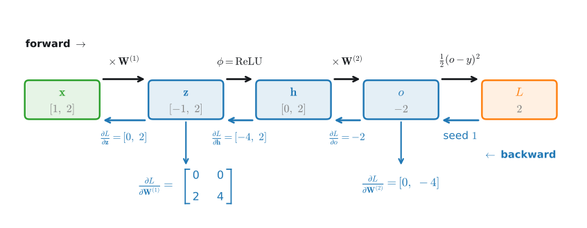
Forward pass builds z, h, o, L; the backward sweep multiplies a gradient back through every node.
Two ways a long product misbehaves
Unstable Gradients
Whether the product grows or shrinks is set by the Jacobians’ scale.
- Factors that contract relevant directions by < 1 \Rightarrow the product shrinks geometrically \Rightarrow vanishing gradient: early layers learn slowly.
- Factors that expand relevant directions by > 1 \Rightarrow the product grows geometrically \Rightarrow exploding gradient: updates can overshoot or produce nonfinite loss.
A constant per-layer factor \rho compounds to \rho^{\,L-\ell}. Only \rho \approx 1 stays usable across depth.
Vanishing: the sigmoid saturates
Unstable Gradients · vanishing
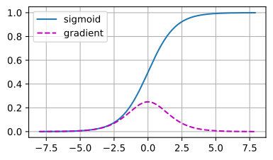
The sigmoid’s derivative peaks at 0.25 and is flat at zero in both tails.
Stack ten such layers and 0.25^{10} \approx 10^{-6}: the bottom layer sees a millionth of the gradient.
ReLU’s derivative is exactly 1 on active coordinates, so the activation does not attenuate gradients there. This property contributes to its use as a common default.
Exploding: one hundred random matrices, entries past 10²⁴
Unstable Gradients · exploding
Multiply one hundred \mathcal{N}(0,1) matrices (for i in range(100): M = M @ randn(4, 4)), exactly what a deep linear stack does to a gradient. The scale of each factor causes rapid growth in the product:
a single matrix [[ 0.37164146 -0.30565897 -0.69504017 -0.3054453 ]
 [-0.32706088  1.5578545   0.259389    1.5199836 ]
 [ 0.24389267 -0.2632121  -0.70784926  0.1288733 ]
 [ 0.48671612 -2.5180435   0.35997918  0.8799593 ]]
after multiplying 100 matrices [[-9.3050529e+23 -6.2406279e+23  2.6926384e+24  1.1626600e+24]
 [ 1.5333718e+24  1.0283879e+24 -4.4371761e+24 -1.9159378e+24]
 [-5.9033706e+23 -3.9592189e+23  1.7082809e+24  7.3762217e+23]
 [-2.3413825e+24 -1.5702974e+24  6.7753473e+24  2.9255421e+24]]
A similarly scaled deep linear network produces gradients of unusable magnitude, for which ordinary optimization typically fails.
Three observable failure modes
Unstable Gradients · in practice
- Loss is NaN from step 1 \to may indicate an exploding initialization or another numerical error.
- Loss spikes mid-training \to may indicate a large gradient on a particular minibatch.
- Loss remains nearly constant \to may indicate vanishing gradients, saturated activations, or a learning rate that is too small.
Random init breaks a hidden symmetry
Unstable Gradients · symmetry
Set every weight in a layer to the same constant c:
- Every hidden unit computes the same function.
- Every unit gets the same gradient.
- After each update the weights are still identical.
The h-unit layer therefore behaves like a single unit under gradient descent.
Gradient descent alone never breaks this tie. Random initialization does; so does dropout. Bias may still start at 0.
02
Variance-Preserving Init
keep the signal’s scale constant through depth
Keep the variance constant, layer to layer
Initialization
For a linear layer o_i = \sum_{j=1}^{n_\textrm{in}} w_{ij} x_j with i.i.d. zero-mean weights (\textrm{Var} = \sigma^2) and inputs (\textrm{Var} = \gamma^2):
\mathbb{E}[o_i] = 0,
\qquad
\textrm{Var}[o_i] = n_\textrm{in}\, \sigma^2\, \gamma^2.
To carry the input’s variance through unchanged (\textrm{Var}[o] = \gamma^2), the only knob is \sigma^2:
\sigma^2 = \frac{1}{n_\textrm{in}}.
Forward and backward disagree, so compromise
Initialization
The same variance count run backward through \mathbf{W}^\top sums over the n_\textrm{out} outputs instead:
\text{forward: } n_\textrm{in}\,\sigma^2 = 1
\qquad
\text{backward: } n_\textrm{out}\,\sigma^2 = 1.
Both cannot hold at once unless n_\textrm{in} = n_\textrm{out}, so Xavier splits the difference by averaging the two fan sizes.
Preserve the activation scale on the way in and the gradient scale on the way out: one \sigma^2, two demands.
Xavier and He: one factor of two apart
Initialization
Xavier / Glorot (2010), for \tanh and sigmoid:
\sigma^2 = \frac{2}{n_\textrm{in} + n_\textrm{out}}.
He / Kaiming (2015), for ReLU:
\sigma^2 = \frac{2}{n_\textrm{in}}.
ReLU zeroes half a symmetric signal, halving its second moment (E[\textrm{ReLU}(z)^2] = \tfrac{1}{2}E[z^2]), so He doubles the weight variance to compensate.
Rule of thumb: Xavier for \tanh/sigmoid, He for ReLU. Both ship as named initializers in most libraries.
The demonstration: 10⁸⁰ vs 10⁻¹⁵ vs flat
Initialization · result
All three regimes in one experiment: push a unit-scale signal through 50 ReLU layers of width 100 and track the second moment E[(h^{(l)})^2] layer by layer, under three weight scales.
- \mathcal{N}(0,1): each layer gains \approx n_\textrm{in}/2 = 50\times, compounding to an astronomical \sim\!10^{80} by layer 50, the exploding regime.
- Xavier: derived for linear layers, off by exactly the rectifier’s \tfrac12 per layer, so the signal vanishes like 2^{-l}, reaching \sim\!10^{-15}.
- He: compensates for the rectifier and holds the scale essentially flat across all fifty layers.
Only the He-initialized stack delivers usable forward signals here. A backward variance calculation gives the same scale under mean-field independence assumptions. Run the sweep yourself in the notebook.
Initialization is necessary but not sufficient
Beyond
A suitable initialization provides usable activation and gradient scales at the start of training. To reach hundreds of layers, modern architecture re-normalizes during training:
- BatchNorm / LayerNorm rescale activations to unit variance each step, lifting the burden off init.
- Residual connections \mathbf{h}^{(\ell+1)} = \mathbf{h}^{(\ell)} + f(\mathbf{h}^{(\ell)}) provide an identity contribution to the gradient, reducing repeated attenuation through residual branches.
We return to both in the chapters on modern CNNs.
Recap
Wrap-up
- A deep gradient is a product of per-layer Jacobians, so it vanishes or explodes without care.
- Vanishing: saturating activations such as sigmoid and tanh attenuate gradients; ReLU avoids positive-side saturation.
- Exploding: over-large weights drive the product, and the loss, to NaN.
- Fix the scale: init weights so \textrm{Var} is preserved, via Xavier (\tanh) and He (ReLU).
- 50-layer experiment: 10^{80} (naive) vs 10^{-15} (Xavier under ReLU) vs flat (He).
- Break hidden-unit symmetry: initialize their weights differently.
- At scale: normalization + residuals + careful init together reach 100+ layers.
Next (the generalization-in-deep-learning section): the model trains, but why does an over-parametrized network generalize at all?