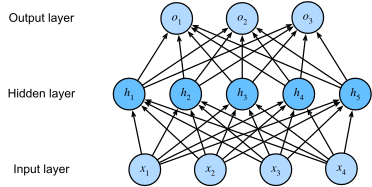
The layers can no longer be merged into one affine map. Composing affine transformations with nonlinear activations produces nonlinear decision surfaces, a pattern used throughout this book.
02
A Nonlinear Example: XOR
a ReLU hidden layer makes the classes linearly separable
A hidden layer makes XOR linearly separable
Why nonlinearity matters
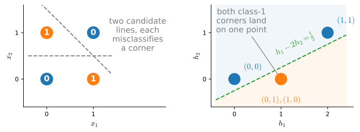
Label each corner of the unit square by whether its coordinates differ. The two classes sit on opposite diagonals (left), so no straight line works.
One hidden layer \mathbf{h} = \operatorname{ReLU}(\mathbf{x}\mathbf{W}^{(1)} + \mathbf{b}^{(1)}) then folds the two label-1 corners onto the same point (right), after which a single line separates them.
Left: XOR in the input space, not linearly separable. Right: after the ReLU hidden map the class-1 corners coincide and a line works.
An MLP represents XOR
XOR · verified
With \mathbf{W}^{(1)} = \left(\begin{smallmatrix}1 & 1\\ 1 & 1\end{smallmatrix}\right), \mathbf{b}^{(1)} = (0,\,{-1}), \mathbf{w}^{(2)} = (1,\,{-2})^\top and a ReLU, pushing all four corners through by hand gives
We constructed these weights; the rest of the book is about having optimization discover such representations. Watch that happen live on the XOR and spiral datasets at the TensorFlow Playground (playground.tensorflow.org).
Universal approximation
Expressive power
Universal approximation theorem. A single hidden layer with enough units can approximate any continuous function on a bounded domain, to arbitrary accuracy, for any non-polynomial \sigma, ReLU included (Cybenko 1989; Leshno et al. 1993).
“Enough units” can be exponentially many; the theorem says a fit exists, not that SGD finds it, nor that it generalizes.
Depth can represent some functions more compactly than a shallow network, trading additional layers for width.
A one-dimensional hinge construction
Expressive power
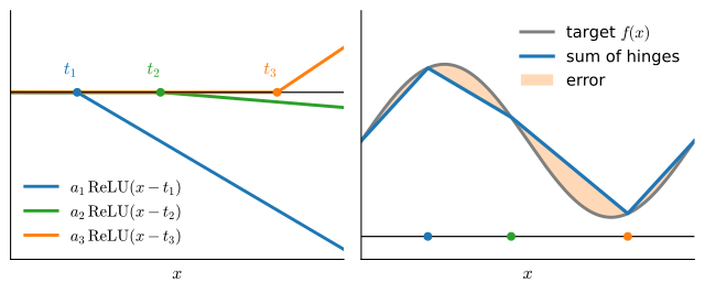
For a one-dimensional construction, each ReLU unit contributes a hingea_k\operatorname{ReLU}(x - t_k): with D units the output is piecewise linear with at most D+1 pieces. Additional joints can refine this polyline approximation.
Three hinges (left) sum to a 4-piece polyline that tracks the smooth target (right); the shaded band is the error.
Depth and the number of linear regions
Expressive power · verified
Evaluate randomly initialized ReLU MLPs on a dense 1-D grid, detect where the slope jumps, and count the linear pieces (mean over 20 draws):
width D
2
4
8
16
bound D+1
3
5
9
17
depth 1
2.6
4.3
7.5
14.4
depth 2
3.5
7.0
13.9
27.4
depth 3
3.6
8.1
22.1
40.1
One layer of width D: at most D+1 pieces, as promised. Each extra layer folds the graph, roughly multiplying the count, the multiplicative-versus-additive gap that can make depth more parameter-efficient.
03
Activation Functions
ReLU, sigmoid, tanh, and when to use each
ReLU: the modern default
Activations
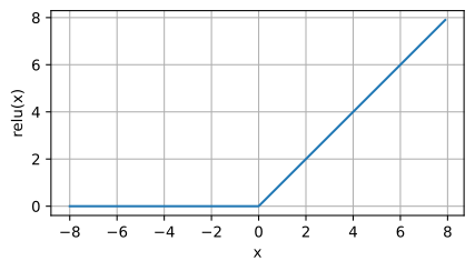
\operatorname{ReLU}(x) = \max(0, x).
x = np.arange(-8.0, 8.0, 0.1)x.attach_grad()with autograd.record(): y = npx.relu(x)d2l.plot(x, y, 'x', 'relu(x)', figsize=(5, 2.5))
The activation retains positive inputs and maps negative inputs to zero:
No right-side saturation: gradient is exactly 1 for x>0.
Cheap: a single comparison, no exponential.
Sparse: about half the units output 0.
ReLU’s gradient: an on/off step
Activations
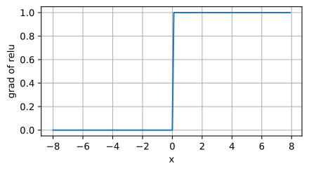
The derivative is a step: 0 on the left, 1 on the right:
\operatorname{ReLU}'(x) = \mathbb{1}[x > 0].
y.backward()d2l.plot(x, x.grad, 'x', 'grad of relu', figsize=(5, 2.5))
Dead ReLU: a unit pushed negative for every example receives zero gradient. LeakyReLU / PReLU, \max(0,x)+\alpha\min(0,x), retain a nonzero negative-side slope.
Sigmoid: squashing into (0, 1)
Activations
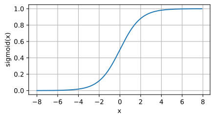
\operatorname{sigmoid}(x) = \frac{1}{1 + e^{-x}}.
with autograd.record(): y = npx.sigmoid(x)d2l.plot(x, y, 'x', 'sigmoid(x)', figsize=(5, 2.5))
This smooth approximation to a threshold is now used mainly at network outputs and in gating mechanisms:
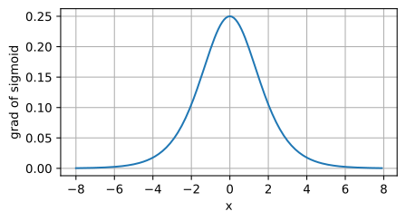
y.backward()d2l.plot(x, x.grad, 'x', 'grad of sigmoid', figsize=(5, 2.5))
The gradient peaks at just 0.25 and vanishes past |x|\gtrsim 5. Even at its best, ten stacked layers attenuate the backward signal by 0.25^{10} \approx 10^{-6}: the vanishing-gradient problem discussed in the numerical-stability section.
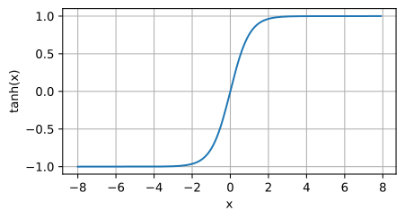
with autograd.record(): y = np.tanh(x)d2l.plot(x, y, 'x', 'tanh(x)', figsize=(5, 2.5))
Same S-shape, but range (-1,1) and zero-centered, which mildly eases optimization. The default inside RNN cells, where bounded activations help.
Still saturates at both tails, so its gradient vanishes just like sigmoid’s.
04
Wrap-up
choosing an activation, plus what comes next
Comparison of activation functions
Reference
Range
Saturates?
Typical use
ReLU
[0, \infty)
left only (can die)
default hidden layer
LeakyReLU / PReLU
\mathbb{R}
no
when ReLU dies
GELU\,x\Phi(x)
\approx\mathbb{R}
barely
BERT, GPT-2-style Transformers
SiLU / SwiGLU
\mathbb{R}
barely
many recent language models
Sigmoid
(0, 1)
both ends
gates, binary output
Tanh
(-1, 1)
both ends
RNN cells
Softmax
simplex
one end
multiclass output
Use ReLU as a simple hidden-layer baseline. Transformer families differ: some use GELU, while many recent language models use gated SiLU/SwiGLU blocks. Use sigmoid / softmax at outputs when the model calls for probabilities.
Recap
Wrap-up
An MLP = affine layers with an elementwise nonlinearity between them.
The nonlinearity is essential; drop it and the stack collapses to one affine map.
XOR is the smallest proof: one ReLU layer re-represents the data so a line works.
One wide hidden layer is a universal approximator: one hinge per unit, \le D+1 pieces; depth multiplies pieces and can represent some functions with fewer parameters.
ReLU is the default; sigmoid and tanh survive in gates, outputs, and RNN cells.
Next (the MLP-implementation section): build one and train it on Fashion-MNIST, from scratch, then in a few high-level API lines.