Concentration and Generalization

Dive into Deep Learning · §27.6

Why averages can be trusted, and when learners cannot
exponential tails · high dimension · uniform convergence · double descent.

Polynomial tails are not enough

Motivation

Chebyshev caps a sample mean’s miss probability at \sigma^2/(nt^2), so its bound for 10^{-6} takes a million times the data of certifying 10^0. The truth for bounded independent data admits an exponential finite-sample bound in n.

The main book bounded test-set error with Hoeffding’s inequality on faith (the generalization-in-classification section). Here we prove it, then follow the same machinery into high dimension and out to generalization itself.

From Chebyshev to Chernoff

one trick: Markov’s inequality, after an exponential

The Chernoff method and exponential moments

Chernoff

Where the MGF M(\lambda)=E[e^{\lambda X}] is finite, Markov’s inequality applied to e^{\lambda X} converts an MGF bound into a tail bound:

P(X \ge t) \;\le\; \inf_{\lambda>0}\; e^{-\lambda t}\, M(\lambda).

For a sum of independent terms the MGF factors, so the exponent grows linearly in n. This is one important concentration route; martingale and bounded-difference methods provide others.

Hoeffding’s lemma: bounded ⇒ sub-Gaussian

Hoeffding

For centered X \in [a,b]: \;E[e^{\lambda X}] \le \exp\bigl(\lambda^2(b-a)^2/8\bigr): an MGF no worse than a Gaussian’s with \sigma = (b-a)/2.

Proof idea. \psi(\lambda) = \log E[e^{\lambda X}] has \psi(0)=\psi'(0)=0, and \psi''(\lambda) is the variance of X under an exponentially tilted distribution, still supported in [a,b], so \psi'' \le (b-a)^2/4 everywhere. Taylor with remainder gives \psi(\lambda) \le \lambda^2(b-a)^2/8. \blacksquare

The one-line fact doing the work: any variable supported in [a,b] has variance at most \bigl(\tfrac{b-a}{2}\bigr)^2.

Hoeffding’s inequality, in four lines

Hoeffding

Independent X_i \in [a,b], \bar X their average:

P\bigl(|\bar X - E[\bar X]| \ge t\bigr) \;\le\; 2\exp\!\left(-\frac{2nt^2}{(b-a)^2}\right).

Proof. Chernoff + independence (MGFs multiply) + the lemma give exponent -\lambda n t + n\lambda^2(b-a)^2/8: a parabola in \lambda, minimized at \lambda = 4t/(b-a)^2 with value -2nt^2/(b-a)^2. The other tail by symmetry; union bound supplies the 2. \blacksquare

No Gaussianity, no variance estimate, no asymptotics: only boundedness and independence, at every finite n.

Bounding test error, now a theorem

Hoeffding

Inverted, Hoeffding is a finite-sample confidence interval: with probability 1-\delta,

|\bar X - E[\bar X]| \;\le\; (b-a)\sqrt{\frac{\log(2/\delta)}{2n}}.

The generalization-in-classification section demanded a test-set error estimate within t=0.01 at \delta = 0.05 and quoted “roughly 18,500 examples.” Solve 2e^{-2nt^2} \le \delta:

n = \frac{\log(2/\delta)}{2t^2} \approx 18{,}445.

A citation is now a theorem, and unlike the Gaussian interval of the statistics section, its coverage is a guarantee at every n, not an asymptote.

Names for the well-behaved: sub-Gaussian and friends

The zoo

X is sub-Gaussian with proxy \sigma^2 if E[e^{\lambda(X-EX)}] \le e^{\lambda^2\sigma^2/2}; Chernoff then gives P(|X-EX| \ge t) \le 2e^{-t^2/(2\sigma^2)}. Three families: Gaussians (proxy \sigma^2, exactly), bounded variables (proxy (b-a)^2/4, the lemma), random signs (proxy 1).

Squares of Gaussians (hence squared norms) are only sub-exponential: Gaussian rate for small deviations, e^{-ct} for large. Bernstein’s inequality covers them and uses the true variance where Hoeffding must assume the worst case.

Numerical comparison of tail bounds

Measured: the fair coin’s exact tail vs. both bounds

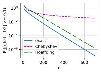
     n      exact  Chebyshev  Hoeffding
    10   7.54e-01   2.50e+00   1.64e+00
   100   5.69e-02   2.50e-01   2.71e-01
  1000   2.73e-10   2.50e-02   4.12e-09
  5000   1.30e-45   5.00e-03   7.44e-44

By n=1000 Chebyshev is off by eight orders of magnitude; by n=5000, about forty-three.

Probability in high dimension

thin shells and orthogonal-by-default directions

A high-dimensional Gaussian is a thin shell

Geometry

\|\mathbf x\|^2 is a sum of d mean-1 terms: a sample-mean problem with sub-exponential summands, and the Bernstein-flavored Chernoff gives

P\!\left(\Bigl|\tfrac{\|\mathbf x\|}{\sqrt d} - 1\Bigr| \ge \varepsilon\right) \;\le\; 2\,e^{-d\varepsilon^2/8}.

The density peaks at the origin, but shell volume grows like r^{d-1}: the mass ends up at r \approx \sqrt d, and the shell’s thickness is O(1), independent of d.

At d=784 a typical draw has norm within a few percent of 28; a draw below norm 14 is rarer than 2e^{-24}. The mode is not the mass.

Random directions are orthogonal by default

Geometry

For a unit \mathbf u, the inner product \langle\mathbf x,\mathbf u\rangle = \sum_i u_i x_i is Hoeffding again (ranges |u_i|, \sum u_i^2 = 1):

P\bigl(|\langle\mathbf x,\mathbf u\rangle| \ge s\bigr) \le 2e^{-s^2/2},

so the cosine is O(1/\sqrt d) with exponentially high probability.

Among n points there are < n^2 pairs, and a union bound flattens every pairwise distance into a (1\pm\varepsilon) band once d \gtrsim \tfrac{8}{\varepsilon^2}\log\tfrac{2n^2}{\delta}: dimension only logarithmic in n. Remember the move: one tail \to many objects, for a logarithmic increase. It is how learning bounds are built.

Measuring the shell

Measured

What fraction of the mass sits in the \pm10\% shell, and what happens to nearest-neighbor contrast:

d=    2:  mass within (1±0.1)·sqrt(d):  14.8%,   NN contrast (d_max-d_min)/d_min = 29.440
d=   20:  mass within (1±0.1)·sqrt(d):  47.6%,   NN contrast (d_max-d_min)/d_min =  1.234
d=  200:  mass within (1±0.1)·sqrt(d):  95.4%,   NN contrast (d_max-d_min)/d_min =  0.239
d= 2000:  mass within (1±0.1)·sqrt(d): 100.0%,   NN contrast (d_max-d_min)/d_min =  0.079

d=2 really is a fuzzy ball (under 15\% in the shell, contrast 29); at d=2000 not one of ten thousand draws left the shell and the farthest of 200 points is only 8\% farther than the nearest.

This is why 1/\sqrt d initialization holds for essentially every draw, and why latent interpolation follows the sphere rather than the chord.

Uniform convergence

the function chosen after the data

The function chosen after the data

The pivot

Hoeffding certifies one fixed function: choose f, then draw the sample. A test set works precisely because it respects this order.

A learner violates it by construction: it searches \mathcal F and returns the \hat f that looks best on the sample it saw, a minimum of fluctuating quantities, selected exactly where the fluctuation flatters. The quantity that must concentrate is the worst case,

\sup_{f\in\mathcal F}\;\bigl|\hat R(f) - R(f)\bigr|.

Test-set reuse is the same trap in different clothes: an analyst who tries many models on one test set is a learner over the class of models tried.

Finite classes: the union bound

Finite classes

For finite \mathcal F, Hoeffding + a union bound over |\mathcal F| bad events: with probability 1-\delta, simultaneously for every f,

\bigl|\hat R(f) - R(f)\bigr| \;\le\; \sqrt{\frac{\log(2|\mathcal F|/\delta)}{2n}}.

Selection freedom enters only through \log|\mathcal F|, under the square root: 2{,}000 hyperparameter configs on a 10{,}000-point validation set move the guarantee only from 0.014 to 0.024; even a pre-registered million, only to 0.030. Adaptive submissions, each chosen after seeing earlier scores, void the union bound entirely: guarantees then degrade much faster (adaptive data analysis).

Rademacher complexity: correlate with coin flips

Infinite classes

Real classes are infinite, so ask a question a learner can act on: how well can \mathcal F correlate with pure noise?

\widehat{\mathfrak R}_S(\mathcal F) = E_{\boldsymbol\varepsilon}\Bigl[\sup_{f\in\mathcal F} \tfrac1n\textstyle\sum_i \varepsilon_i f(\mathbf x_i)\Bigr], \qquad R(f) \le \hat R(f) + 2\,\mathfrak R_n(\mathcal F) + \sqrt{\tfrac{\log(1/\delta)}{2n}}.

A class that can chase coin flips can chase the noise in real labels; one that cannot has trustworthy empirical risks.

The factor 2 is symmetrization: a ghost sample plus the swap trick conjures the random signs out of a statement that contains none; McDiarmid lifts it to high probability.

The linear class: capacity is Br/√n

The linear class

For \mathcal F = \{\mathbf x \mapsto \langle\mathbf w,\mathbf x\rangle : \|\mathbf w\| \le B\} on data with \|\mathbf x_i\| \le r, the supremum is Cauchy–Schwarz in closed form, and independent signs kill the cross terms:

\widehat{\mathfrak R}_S = \frac Bn\,E\Bigl\|\sum_i \varepsilon_i \mathbf x_i\Bigr\| \;\le\; \frac{B\,r}{\sqrt n}.

The dimension d is absent from this bound: linear classes with different feature counts have the same bound when the input and weight radii match. Feature changes can alter those radii, and a radius chosen after fitting needs a data-dependent analysis.

Coin flips in code

Measured

Monte-Carlo Rademacher complexity of the unit-norm linear class, plus the Zhang phenomenon in miniature, an interpolating class fed 2{,}000 sets of coin flips:

Monte-Carlo Rademacher complexity  = 0.1390
bound B*r/sqrt(n)                  = 0.1414
correlation of min-norm fits with coin flips = 1.0000
norm it costs: mean ||w|| = 1.00;  implied capacity bound B*r/sqrt(n) = 1.41

The bound 0.1414 is within 2\% of the truth. The interpolating class scores correlation 1.0000 on every flip set, and its own printout shows the norm it needed: the smallest linear class containing those fits has Br/\sqrt n \approx 1.41 > 1. Vacuous, as it must be.

When uniform-convergence bounds are vacuous

Limits

Zhang et al. trained standard architectures to zero training error on CIFAR-10 with randomly shuffled labels: the class “this architecture, trained by SGD” correlates perfectly with coin flips, so its Rademacher complexity is \approx 1 and the bound certifies nothing.

This is a fact about these bounds, which take uniform convergence over the entire representable class. The same network generalizes on real labels, so a whole-class bound misses properties of the data, algorithm, and reached solution.

Solution norm is one useful diagnostic. The final section studies it in a controlled random-features model; it is not a complete theory of deep networks.

Interpolation and double descent

a controlled random-features example

Beyond the U-curve

Double descent

The U-curve is a heuristic, not a consequence required by bias–variance or uniform convergence. In some interpolating problems, test error peaks near the interpolation threshold and then falls again as the model grows.

The smallest model that shows it: random-features regression. \phi(\mathbf x) = \mathrm{ReLU}(\mathbf V\mathbf x) with \mathbf V random and frozen, the head fit by the pseudoinverse: least squares below the threshold, the minimum-norm interpolant above it.

The peak is a conditioning event

Double descent

At p = n the feature matrix is square and almost never well invertible: interpolation divides the labels’ noise by a tiny \sigma_{\min}, the norm explodes, the test error spikes.

Beyond it, nested features give an exact monotonicity: any interpolant at p pads with a zero to one at p+1, so

\bigl\|\mathbf w^{(p+1)}_{\min}\bigr\| \;\le\; \bigl\|\mathbf w^{(p)}_{\min}\bigr\| :

more nested features let the minimum-norm interpolant get smaller. This helps explain the experiment below, but Br/\sqrt n also contains the feature radius r, and a data-dependent fitted radius needs localized analysis.

Double descent in twenty-six lines

Measured: forty noisy points, ReLU random features, swept through p = n

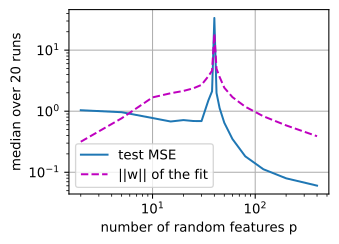
p=  2  test MSE=   1.0378  train MSE= 8.67e-01  ||w||=   0.32
p=  5  test MSE=   0.9627  train MSE= 7.70e-01  ||w||=   0.77
p= 10  test MSE=   0.7728  train MSE= 4.64e-01  ||w||=   1.68
p= 15  test MSE=   0.6782  train MSE= 2.81e-01  ||w||=   1.97
p= 20  test MSE=   0.7156  train MSE= 1.54e-01  ||w||=   2.15
p= 25  test MSE=   0.6905  train MSE= 8.10e-02  ||w||=   2.37
...
p= 50  test MSE=   0.6466  train MSE= 7.80e-30  ||w||=   2.42
p= 60  test MSE=   0.3507  train MSE= 5.29e-30  ||w||=   1.70
p= 80  test MSE=   0.1824  train MSE= 5.00e-30  ||w||=   1.18
p=120  test MSE=   0.1121  train MSE= 6.61e-30  ||w||=   0.83
p=200  test MSE=   0.0796  train MSE= 8.08e-30  ||w||=   0.59
p=400  test MSE=   0.0604  train MSE= 8.04e-30  ||w||=   0.39

Norm tracks the second descent here

Double descent

Read the sweep’s numbers against the mechanism: at p = n = 40 the train error hits 10^{-28} (exact interpolation) and the test error erupts to 33.6, fifty times the classical minimum, with \|\mathbf w\| = 18.5. Then the norm falls monotonically to 0.39 and the test error follows it down to 0.060 at p=400: ten times better than the best underparameterized model, from a model that fits noisy data exactly.

Past the threshold the train error is zero up to floating point everywhere, so training error does not distinguish the p=42 and p=400 fits. Their solution norms differ and correlate with test error in this experiment; the Rademacher bound alone does not predict the curve because feature norms and data-dependent selection also matter.

Benign overfitting in linear models

Double descent

The p=400 model reproduces every corrupted label exactly, yet tests best. The min-norm solution splits across the spectrum: a few strong singular directions carry the signal, and minimizing the norm spreads the interpolated noise across the many weak directions, where it barely contaminates new predictions.

Under suitable covariance spectra, interpolation can be benign when the spectrum offers a few strong directions for the signal and a large reservoir of weak ones to absorb the noise.

Made exact for linear regression (two effective ranks of the covariance); for deep networks, where the features are learned and reshape the spectrum, the theory is instructive but open.

Recap

Wrap-up

Chernoff: Markov on e^{\lambda X}; independent sums factor the MGF → exponential tails.
Hoeffding: 2e^{-2nt^2/(b-a)^2} turns the generalization-in- classification section’s 18,500-example quote into a theorem, valid at every finite n.
High dimension: thin shells, orthogonal-by-default directions.

Uniform convergence: \log|\mathcal F| for a pre-registered pool, then Rademacher; for a linear class with fixed input and weight radii the bound is Br/\sqrt n, with no explicit parameter count.
Whole-class bounds can be vacuous for models able to interpolate random labels (Zhang et al.).
Double descent: a \sigma_{\min} spike, then the min-norm interpolant’s norm falls, and overfitting can be benign.

Hoeffding certifies a fixed test-set estimate, and the union bound extends the result to a fixed finite collection of models. For linear classes, the resulting capacity measure depends on the norm.