Single Variable Calculus

Dive into Deep Learning · §25.1

Local approximation for optimization
the derivative · gradient descent · curvature · Taylor · corners.

Derivatives and Optimization

Motivation

Training collects the weights in a vector \mathbf{w} and minimizes a loss L(\mathbf{w}). When a direct solution is unavailable, iterative methods use local derivatives.

Holding every weight but one fixed gives a curve f(x) in a single variable:

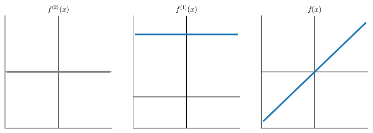
The derivative determines the local direction and rate of decrease.
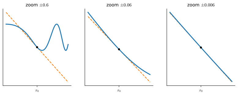
Zoom in on a smooth curve and it flattens onto a line, the tangent at the base point.

01

The derivative

zooming in, secants, and the tangent slope

Local Linear Approximation

The derivative

On a sufficiently small neighborhood, a differentiable function is approximated by its tangent line. The tangent slope is the derivative.

image/svg+xml Matplotlib v3.10.8, https://matplotlib.org/

From secant to tangent

The derivative

The difference quotient is the slope of the secant through two nearby points:

\frac{f(x+\epsilon) - f(x)}{\epsilon}.

As \epsilon \to 0 the second point slides in and the secant rotates into the tangent, whose limiting slope is the derivative f'(x).
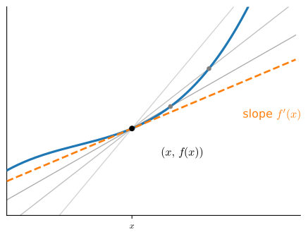
As \epsilon \to 0 the secant through (x,f(x)) and (x+\epsilon,f(x+\epsilon)) rotates into the tangent, whose slope is f'(x).

Convergence of the Difference Quotient

The derivative

For f(x) = x^2 + 1701(x-4)^3 at x=4, the secant slope approaches 8 as \epsilon shrinks:

# Define our function
def f(x):
    return x**2 + 1701*(x-4)**3

# Slope of the secant through x=4, for shrinking epsilon
for epsilon in [0.1, 0.001, 0.0001, 0.00001]:
    print(f'epsilon = {epsilon:.5f} -> {(f(4+epsilon) - f(4)) / epsilon:.5f}')
epsilon = 0.10000 -> 25.11000
epsilon = 0.00100 -> 8.00270
epsilon = 0.00010 -> 8.00012
epsilon = 0.00001 -> 8.00001

Finite differences approach the limit; autograd applies differentiation rules without \epsilon:

autograd: f'(4) = 8.0

The small-change identity

The derivative

Rearranging the limit gives the small-change identity:

f(x+\epsilon) \approx f(x) + \epsilon\,f'(x).

The derivative gives the first-order output change produced by an input perturbation. Differentiation rules, gradient descent, and Taylor series all use this local approximation.

02

Linear approximation & descent

the tangent line becomes a step downhill

The tangent line is the best local model

Optimization

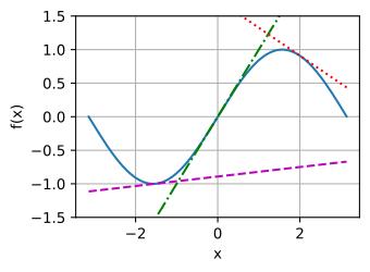
Read as a function of the displacement, f(x+\epsilon) \approx f(x) + \epsilon f'(x) is the tangent line at x, the best straight-line model of f nearby.

For three points of \sin (using \tfrac{d}{dx}\sin = \cos), each tangent is accurate locally and diverges from the curve farther away.
The gradient-descent step

Optimization

Choose \epsilon = -\eta\,f'(x) with step size \eta > 0. The first-order model then decreases by

\approx \eta\,[f'(x)]^2 \ge 0.

Whatever the sign of f', stepping against it lowers f, by an amount proportional to the slope squared. Iterating is gradient descent, x_{t+1} = x_t - \eta f'(x_t).

image/svg+xml Matplotlib v3.10.8, https://matplotlib.org/

The descent lemma

Optimization

image/svg+xml Matplotlib v3.10.8, https://matplotlib.org/

If the slope is L-Lipschitz, f(x) + f'(x)s + \tfrac{L}{2}s^2 is a quadratic upper bound that equals the function at the base point.

Stepping to the ceiling’s minimizer (the gradient step with \eta = 1/L) drops f by at least \tfrac{1}{2L}[f'(x)]^2:

f\!\left(x - \eta f'(x)\right) \le f(x) - \eta\!\left(1 - \tfrac{L\eta}{2}\right)[f'(x)]^2.

A strict decrease for every 0 < \eta < 2/L.

Gradient Descent for Different Step Sizes

Optimization
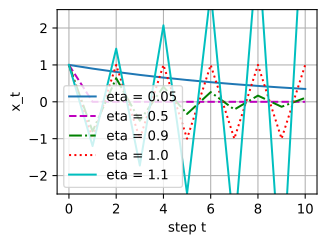
eta = 0.05 -> x_10 = +0.34868
eta = 0.50 -> x_10 = +0.00000
eta = 0.90 -> x_10 = +0.10737
eta = 1.00 -> x_10 = +1.00000
eta = 1.10 -> x_10 = +6.19174

Gradient descent on f(x) = x^2 (L = 2) from x_0 = 1, ten steps each.

The cases are slow convergence (\eta{=}0.05), one-step convergence (\tfrac12{=}1/L), oscillatory convergence (0.9), a two-cycle (1.0), and divergence (1.1). The guarantee ends at \eta = 2/L.

03

Curvature & Taylor

the second derivative and the best polynomial

The second derivative is curvature

Curvature

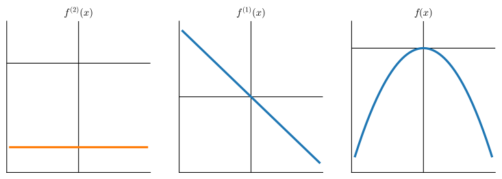
At a stationary point (f'=0) the sign of f'' decides the shape: up into a minimum, down into a maximum, flat is undecided. This is the second-derivative test.
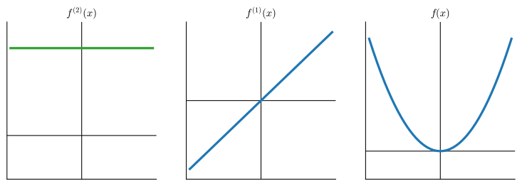
f'' > 0: slope rising, a bowl, local min.

f'' < 0: slope falling, a dome, local max.

f'' = 0: slope constant, a line, inconclusive.

The Mean Value Theorem

Curvature

The theorem relates a derivative of f at an interior point to the average rate of change over an interval:

f'(\xi) = \frac{f(b) - f(a)}{b - a}\quad\text{for some }\xi \in (a,b).

It shows how the sign of the derivative determines where f is increasing and also supports the Taylor remainder bound.
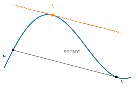
Some interior tangent runs parallel to the chord through the endpoints.

Quadratic Approximation and Newton’s Method

Curvature

Matching value, slope, and curvature gives the local quadratic Taylor model. When f''(x_t)>0, minimizing that model proposes Newton’s step x_{t+1}=x_t-f'(x_t)/f''(x_t).

The proposal need not improve the original function far from a solution; damping or a trust region controls the step when the local model is unreliable.
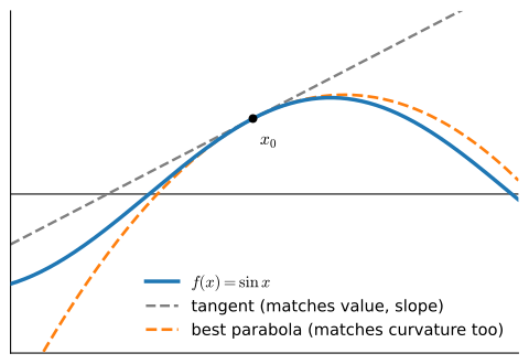
The tangent matches value and slope; the best parabola also matches curvature.

Quadratic Convergence of Newton’s Method

Curvature

On f(x) = \tfrac14 x^4 - x, Newton’s method solves f'(x) = x^3 - 1 = 0 from x_0 = 2. Read the error column’s exponents: 10^{-2} \to 10^{-4} \to 10^{-8}.

# Newton's method on f(x) = x^4/4 - x: solve f'(x) = x^3 - 1 = 0, root x* = 1
x = 2.0
for t in range(6):
    print(f't = {t}: x = {x:.12f}, error = {abs(x - 1):.1e}')
    x = x - (x**3 - 1) / (3 * x**2)  # x - f'(x) / f''(x)
t = 0: x = 2.000000000000, error = 1.0e+00
t = 1: x = 1.416666666667, error = 4.2e-01
t = 2: x = 1.110534409842, error = 1.1e-01
t = 3: x = 1.010636768405, error = 1.1e-02
t = 4: x = 1.000111557304, error = 1.1e-04
t = 5: x = 1.000000012443, error = 1.2e-08

For this run, each step roughly squares the previous error. Under the local regularity assumptions stated in the text, this is quadratic convergence. Fixed-step gradient descent on a smooth, strongly convex neighborhood instead has linear convergence.

The Taylor Polynomial Matches n Derivatives

Curvature

Matching the first n derivatives at x_0 gives the Taylor polynomial

P_n(x) = \sum_{i=0}^{n} \frac{f^{(i)}(x_0)}{i!}(x-x_0)^i.

For e^x at x_0 = 0, raising the degree visibly tightens the fit to the curve.
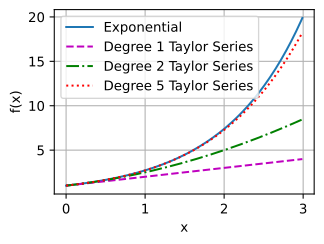
Taylor Remainder by Polynomial Degree

Curvature

The Lagrange remainder makes “the approximation improves near x_0” quantitative: the error shrinks like |x - x_0|^{n+1}, so halving the window should divide the worst error by 2^{n+1}:

n = 1: max error 2.1e-02 (h = 0.2) vs 5.2e-03 (h = 0.1), ratio = 4.1, prediction 2^2 = 4
n = 2: max error 1.4e-03 (h = 0.2) vs 1.7e-04 (h = 0.1), ratio = 8.2, prediction 2^3 = 8
n = 3: max error 6.9e-05 (h = 0.2) vs 4.3e-06 (h = 0.1), ratio = 16.3, prediction 2^4 = 16

The measured ratios match the predicted 4, 8, and 16. Each additional matched derivative increases the error order by one.

Smooth is not analytic

Curvature

Smoothness alone does not justify an infinite Taylor representation. The function f(x) = e^{-1/x^2} is smooth everywhere, yet every derivative at 0 vanishes.

Its Taylor series at 0 is identically zero: it converges on the whole line, but to the zero function, agreeing with f only at the origin. Convergence of the series is not convergence to f.
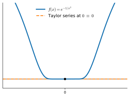
e^{-1/x^2} (solid) against its Taylor series at 0 (the zero line): smooth \ne analytic.

04

When the tangent fails

corners, subgradients, and stochastic training

Corners: no single tangent

Nonsmooth

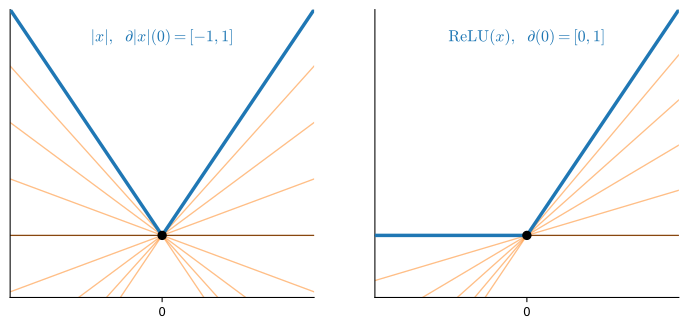
At each corner the one-sided slopes disagree; the subdifferential is the fan of all lines that stay below the graph.

At a corner (|x|, \mathrm{ReLU}) the one-sided slopes differ, so no single tangent exists. The subdifferential collects every valid slope:

\partial|x|(0) = [-1,1],\quad \partial\,\mathrm{ReLU}(0) = [0,1].

Optimality relaxes from f'(x)=0 to the inclusion 0 \in \partial f(x).

The split is in the difference quotient

Nonsmooth

The one-sided quotients of |x| at 0 are constants that never agree: +1 from the right, -1 from the left, so there is no limit to take. At the corner, autograd returns a convention-dependent value:

# One-sided difference quotients of |x| at 0: constants, no limit needed
epsilon = 1e-4
print(f'right quotient: {(abs(epsilon) - abs(0)) / epsilon:+.1f}, '
      f'left quotient: {(abs(-epsilon) - abs(0)) / -epsilon:+.1f}')

# What autograd returns at the corner, where no derivative exists
for name, fn in [('d|x|/dx', np.abs), ("ReLU'", npx.relu)]:
    x = np.array(0.0)
    x.attach_grad()
    with autograd.record():
        y = fn(x)
    y.backward()
    print(f"{name} at 0: autograd returns {float(x.grad):.1f}")
right quotient: +1.0, left quotient: -1.0
d|x|/dx at 0: autograd returns 0.0
ReLU' at 0: autograd returns 0.0

That gap is the corner: the two-sided derivative exists only when the one-sided slopes coincide. The 0 autograd returns is a convention, one fixed element of the set defined next.

The chain rule at a kink

Nonsmooth

At each kink, autograd returns one fixed element of the subdifferential (\mathrm{ReLU}'(0) = 0) and chains it through. But g(x) = \mathrm{ReLU}(x) - \mathrm{ReLU}(-x) is the identity, whose only correct slope at 0 is 1. Run it:

# g(x) = relu(x) - relu(-x) is the identity, so the true slope at 0 is 1
x = np.array(0.0)
x.attach_grad()
with autograd.record():
    g = npx.relu(x) - npx.relu(-x)
g.backward()
print(f"autograd: g'(0) = {float(x.grad):.1f}  (true slope: 1.0)")
autograd: g'(0) = 0.0  (true slope: 1.0)

Autograd reports slope 0 for the identity function: the chained convention 0 + 0 is not a subgradient of g at 0 at all, only an element of a conservative field.

Nonsmooth Points in Stochastic Training

Nonsmooth

The incorrect chained value occurs only at a kink. The set of kinks is often treated heuristically as a measure-zero set.

Under a continuous sampling distribution, a fixed measure-zero set is hit with probability zero. Training iterates are data-dependent, however, and can encounter kinks. Conservative-field convergence results cover many definable networks under their stated boundedness, step-size, and noise assumptions; they are not an unconditional guarantee for arbitrary nonsmooth training.

Derivatives organize local prediction and optimization

Wrap-up

  • Derivative = slope the curve flattens onto = limit of secants.
  • The small-change identity f(x+\epsilon)\approx f(x)+\epsilon f'(x) organizes the derivative rules and local optimization arguments in this section.
  • First-order term → gradient descent x \leftarrow x - \eta f'(x), safe for \eta < 2/L.
  • Second derivative = curvature; its sign is the min/max test.
  • Quadratic term → Newton’s method x_{t+1} = x_t - f'(x_t)/f''(x_t).
  • At corners, a subgradient may define optimality, while autodiff follows an implementation convention that requires separate convergence assumptions.