Policy Gradient

Dive into Deep Learning · §14.5

Policy gradient
a parameterized policy · the log-derivative identity · model-free gradient estimation · bias and variance diagnostics

Differentiate the Return Itself

No model (:numref:sec_valueiter had one), no expert (:numref:sec_imitation), and no value function either: write the policy as a differentiable function of \theta and ascend J(\theta).

\pi_\theta(a \mid s) = \frac{e^{\theta_{s,a}}}{\sum_{a'} e^{\theta_{s,a'}}}, \qquad J(\theta) = E_{\tau \sim P(\cdot;\, \theta)} \big[ R(\tau) \big]

  • one free preference \theta_{s,a} per pair: ActorCritic.tabular, reused from :numref:sec_imitation
  • softmax keeps every probability positive: exploration built in early; support alone is not a visitation guarantee
  • calm ice, and no time limit, both named as assumptions: the estimator isolates the policy distribution from the environment dynamics

The Score Function, Verified

\frac{\partial \log \pi_\theta(a \mid s)}{\partial \theta_{s,b}} = \mathbf{1}(b = a) - \pi_\theta(b \mid s)

rng = np.random.default_rng(0)
theta = jnp.asarray(rng.standard_normal((16, 4)))   # a generic table
score = jax.grad(lambda th: jax.nn.log_softmax(th[6])[2])(theta)
hand = jnp.zeros_like(theta).at[6].set(-jax.nn.softmax(theta[6]))
hand = hand.at[6, 2].add(1.0)
print(bool(jnp.allclose(score, hand, atol=1e-6)))
True

Automatic differentiation verifies the analytic score identity in both framework implementations.

The Log-Derivative Trick

R(\tau) does not depend on \theta; only the trajectory’s probability does:

\nabla_\theta J(\theta) = \sum_\tau R(\tau)\, \nabla_\theta P(\tau; \theta) = \sum_\tau P(\tau; \theta)\, R(\tau)\, \nabla_\theta \log P(\tau; \theta)

\nabla_\theta \log P(\tau; \theta) = \sum_t \nabla_\theta \log \pi_\theta(a_t \mid s_t)

The transition terms have zero gradient because the kernel does not depend on the policy parameters. Sampling n trajectories gives REINFORCE:

\hat u = \frac{1}{n} \sum_i R(\tau_i) \sum_t \nabla_\theta \log \pi_\theta(a_t^i \mid s_t^i)

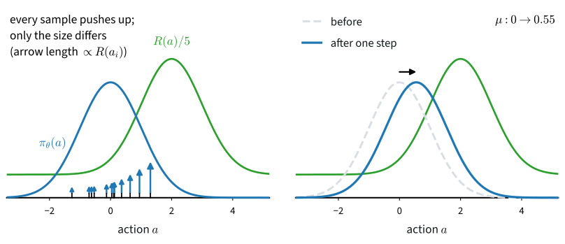
One Step, Drawn

All rewards in this example are positive, so every sampled action receives a positive weight. :numref:sec_baselines introduces centered weights that can be positive or negative.

Trajectories Become Data

def rollout(env, policy, num_episodes, rng):
    """Collect complete episodes from `policy(obs, rng) -> action` as a
    Batch; `term` records `terminated`, never `truncated` (:numref:`sec_mdp`).

    All sampling runs through the one numpy generator `rng`."""
    cols, ep_ends = [[] for _ in range(5)], []
    for _ in range(num_episodes):
        obs, done = env.reset()[0], False
        while not done:
            act = policy(obs, rng)
            next_obs, reward, terminated, truncated, _ = env.step(act)
            done = terminated or truncated
            for col, val in zip(cols, (obs, act, reward, next_obs,
                                       float(terminated))):
                col.append(val)
            obs = next_obs
        ep_ends.append(len(cols[0]))
    obs, act, rew, next_obs, term = (np.asarray(c) for c in cols)
    return Batch(obs, act, rew.astype(np.float32), next_obs,
                 term.astype(np.float32), np.asarray(ep_ends))

term records terminated, not truncated; later algorithms use the same distinction.

REINFORCE on the Calm Lake

def train_reinforce(ac, seed, steps, num_updates=256, batch_episodes=16):
    """REINFORCE: a fresh batch from the current policy, every step of a
    trajectory weighted by that trajectory's return, one ascent step."""
    rng = np.random.default_rng(seed)      # one stream for all sampling
    env.reset(seed=seed)
    for _ in range(num_updates):
        batch = rollout(env, ac.act, batch_episodes, rng)
        R = batch.episode_returns(gamma)
        d2l.policy_step(ac, batch,
                        np.repeat(R, np.diff(batch.ep_ends, prepend=0)))
        steps.append(len(batch))
        yield float(R.mean())
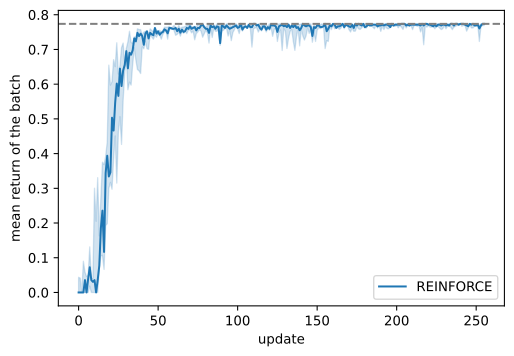
Updates are zero until the first successful trajectory. The mean return then increases and stabilizes below \gamma^5 = 0.774.

What It Costs

The on-policy derivation requires trajectories from the current policy.

update at which the batch mean first reaches 0.7: [24 27 30]
environment steps spent by that update:  [3210 3789 4287]
environment steps spent by the full run: [26058 26582 27472]

Learning requires about 3,000–4,500 steps, while the complete run uses about 27,000 because every update collects new data. :numref:sec_qlearning’s slippery-map run: 95,569 steps.

Unbiased, Measured

On 16 states J(\theta) = [(I - \gamma P^\pi)^{-1} r^\pi]_{s_0} is a differentiable linear solve: autograd gives the exact gradient.

n=  4: zero estimates  3/50, cos(mean, exact) = 0.93, single-estimate relative error = 3.64
n= 16: zero estimates  0/50, cos(mean, exact) = 0.97, single-estimate relative error = 1.74
n= 64: zero estimates  0/50, cos(mean, exact) = 1.00, single-estimate relative error = 0.94

The mean estimate aligns with the exact gradient, while individual batches have substantial error that decreases as 1/\sqrt{n}. :numref:sec_baselines uses the same exact-gradient reference.

Recap

  • The log-derivative identity expresses \nabla_\theta J as an expectation over trajectory scores; kernel terms have zero derivative.
  • REINFORCE weights each trajectory score by its return. Its sample mean is compared with the exact \nabla_\theta J in this example.
  • Policy gradient theorem: the same gradient over the discounted occupancy, Q^\pi against the score.
  • On-policy methods collect fresh data after every update.
  • Because J(\theta) is not concave, gradient ascent may reach only a stationary point rather than a globally optimal policy \pi^*.
  • Noise falls only as 1/\sqrt{n}: variance reduction is :numref:sec_baselines.