@d2l.add_to_class(d2l.Batch)
def backward_scan(self, x, factor):
    """y_t = x_t + factor * y_{t+1}, restarted at every episode boundary."""
    y = np.zeros_like(x)
    for ep in self.episodes():
        running = 0.0
        for t in reversed(range(ep.start, ep.stop)):
            running = x[t] + factor * running
            y[t] = running
    return y

@d2l.add_to_class(d2l.Batch)
def reward_to_go(self, gamma):
    """G_t: the discounted return of the rest of its episode, by one scan."""
return self.backward_scan(self.rew, gamma)Variance Reduction for Policy Gradients
Dive into Deep Learning · §14.6
Baselines, advantages and variance reduction
one zero-mean identity · reward-to-go, baselines, control variates · centering is a baseline, dividing by \sigma is a step size · measured against the exact gradient
One Zero-Mean Identity
\sum_a \pi_\theta(a \mid s)\, \nabla_\theta \log \pi_\theta(a \mid s) = \nabla_\theta \sum_a \pi_\theta(a \mid s) = \nabla_\theta 1 = 0
Condition on the prefix: anything already determined at s_t has a mean-zero product with the score,
E\big[ c\ \nabla_\theta \log \pi_\theta(a_t \mid s_t) \big] = 0.
Multiply a score by such a c, or subtract it from the weight, and the expectation is unchanged. Reward-to-go, state baselines, and leave-one-out baselines are applications of this identity.
Reward-to-Go: One Scan
Past rewards have zero expected product with the score at t, so they can be removed:
\hat u = \frac1n \sum_i \sum_t \hat G^i_t\, \nabla_\theta \log \pi_\theta(a^i_t \mid s^i_t), \qquad \hat G_t = \sum_{t'\ge t} \gamma^{t'-t} r_{t'}.
GAE will be this same scan, run on TD errors with factor \gamma\lambda.
A Baseline Is a Control Variate
To estimate E[X]: subtract anything whose mean you know,
X_c = X - c\,(Y - E[Y]), \qquad c^* = \frac{\mathrm{Cov}(X,Y)}{\mathrm{Var}(Y)} \ \Rightarrow\ \mathrm{Var} = (1-\mathrm{corr}^2)\,\mathrm{Var}(X).
At \mathrm{corr} = 0.9 the variance falls by a factor of about five.
Here: X = \hat G_t \nabla_\theta \log \pi_\theta(a_t \mid s_t), \ Y = \nabla_\theta \log \pi_\theta(a_t \mid s_t), \ E[Y] = 0 by the lemma. Choosing b(s_t) is choosing c; the optimum is c^*, state by state.
Effect of a Baseline
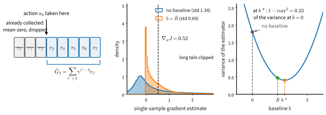
Drop the past; subtract b = E[R] and the std halves (1.34 \to 0.69); the parabola’s optimum b^\star leaves 1 - \mathrm{corr}^2 = 0.23 of the variance.
The Advantage, and a Learned Baseline
A natural b(s) is the value function, which makes the weight a sampled advantage (:numref:sec_valueiter defined it).
\hat V(s_t) \leftarrow \hat V(s_t) + \alpha_V\,(\hat G_t - \hat V(s_t)), \qquad \textrm{weight} = \hat G_t - \hat V(s_t) \approx A^{\pi_\theta}.
This section uses Monte Carlo regression; the next chapter introduces bootstrapped actor–critic targets.
Dependence Conditions Determine Baseline Bias
Leave-one-out: b_i = \frac{1}{n-1}\sum_{j \neq i} R(\tau_j), independent of trajectory i: exactly unbiased. It is \frac{n}{n-1} \times centering, and it is RLOO.
What do you divide the summed loss by?
episode lengths [ 8 20  8 11], successes 3
    episodes: |grad| = 0.868, cos to episodes = 1.000
  own length: |grad| = 0.082, cos to episodes = 0.937
 total steps: |grad| = 0.074, cos to episodes = 1.000
  a constant: |grad| = 0.109, cos to episodes = 1.000
Three pure rescalings, one changed direction: the Dr. GRPO / token-loss debate on a four-episode batch.
Normalized Returns Became GRPO
A_j = \frac{r_j - \mu}{\sigma + 10^{-8}}
- prompt \leftrightarrow start state; group of K responses \leftrightarrow batch of trajectories
- group mean = a per-prompt baseline without a value network
- dividing by \sigma: a per-prompt step-size rescaling, not a baseline (Dr. GRPO’s objection)
Five Estimators at a Frozen Theta
The policy is held fixed, and its exact gradient provides the reference against which every estimator is measured.
        return: cos(mean, exact) = 0.98, relative variance =   11.1
  reward-to-go: cos(mean, exact) = 0.97, relative variance =   10.6
      centered: cos(mean, exact) = 0.98, relative variance =    7.1
    normalized: cos(mean, exact) = 0.97, relative variance =    6.9
exact baseline: cos(mean, exact) = 0.98, relative variance =    5.3
The matching cosines confirm that baselines preserve the expected gradient. Centering reduces variance by one third, and the exact state baseline nearly halves it. Dividing by \sigma gives no further reduction, while reward-to-go helps little because a terminal-only reward leaves no earlier rewards to omit.
Estimator Comparison
All variants use the same \alpha, plain SGD, matched batches, and twenty seeds; only the score weights differ.
          return: updates to 90%: median  60.0, fastest  26, slowest  92
                  mean |step| over the first 40 updates: 0.20
    reward-to-go: updates to 90%: median  40.0, fastest  22, slowest  95
                  mean |step| over the first 40 updates: 0.38
        centered: updates to 90%: median  58.0, fastest  43, slowest 108
                  mean |step| over the first 40 updates: 0.15
      normalized: updates to 90%: median  30.0, fastest   8, slowest  72
                  mean |step| over the first 40 updates: 0.76
learned baseline: updates to 90%: median  40.5, fastest  22, slowest  84
mean |step| over the first 40 updates: 0.32- Normalization learns fastest here, but its updates are about 5\times those of centering and 2\times those of reward-to-go.
- Subtracting \mu gives a baseline. Dividing by \sigma + 10^{-8} changes the per-batch step size rather than the baseline.
- At fixed \alpha, performance depends on both variance and update scale.
How To Read RL Curves
- every band is wide: slowest seed > 2\times the fastest, same variant, only the seed changed
- individual seeds can reverse an apparent ordering
- twenty seeds support the broad ordering rather than precise digits; report ranges and ratios
- several seeds, matched hyper-parameters, medians, spread :cite:
Henderson.Islam.Bachman.ea.2018,Agarwal.Schwarzer.Castro.ea.2021,Engstrom.Ilyas.Santurkar.ea.2020
Recap
- One lemma: the score has zero conditional mean; anything determined at s_t can weight or offset it, bias-free.
- Reward-to-go, baselines, the optimal c^*, the learned \hat V: four uses of the identity.
- A baseline is a control variate; the factor (1-\mathrm{corr}^2) quantifies its variance reduction.
- Centering is a baseline; \div\,\sigma is a step size; leave-one-out is exact; the loss divisor is a fourth estimator choice. GRPO is this section at scale.
- Entropy decreases from \ln 4 to about 0.8 nats without an explicit constraint; :numref:
sec_ppocontrols policy change.