What makes deep-net optimization hard risk vs. empirical risk · where gradients vanish · curvature and noise · the edge of stability
An optimizer is three decisions
The chapter’s frame
A descent direction — which way is “down”? Depends on which norm measures the step. Euclidean → the negative gradient. Other norms → other algorithms (as developed for Muon).
A step size over time — how far to trust the local slope, and how that trust changes over a run (schedules, warmup).
A way of living with noise — every gradient is a minibatch estimate; batch size and averaging set the noise level.
Every method in this chapter, GD through Muon, is one way of making these three decisions.
Optimization vs. learning
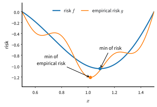
Optimization minimizes the empirical risk (training loss). Learning wants low risk (expected loss on the population). The optimizer only ever sees the former — and the two minima sit in different places, which no optimizer can fix:
The empirical-risk and population-risk minima need not coincide, so lower training loss does not guarantee lower population loss.
Local minima
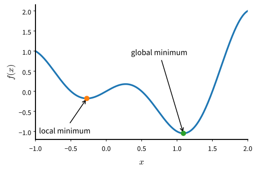
f(x) = x \cos(\pi x) has a local minimum that is not global. Near it, the gradient goes to zero — the signal cannot tell the two apart:
The derivative vanishes at both local and global minima; local gradient information alone does not distinguish them.
Noise can knock the iterate out of a shallow basin — minibatch variance supplies exactly that.
Saddle points
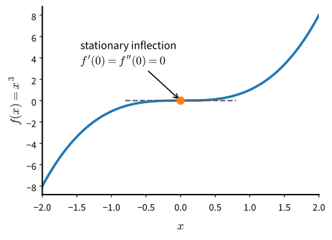
1D: f(x) = x^3 has f'(0) = 0, yet no minimum:
At the origin, the first and second derivatives vanish even though the cubic has no extremum.
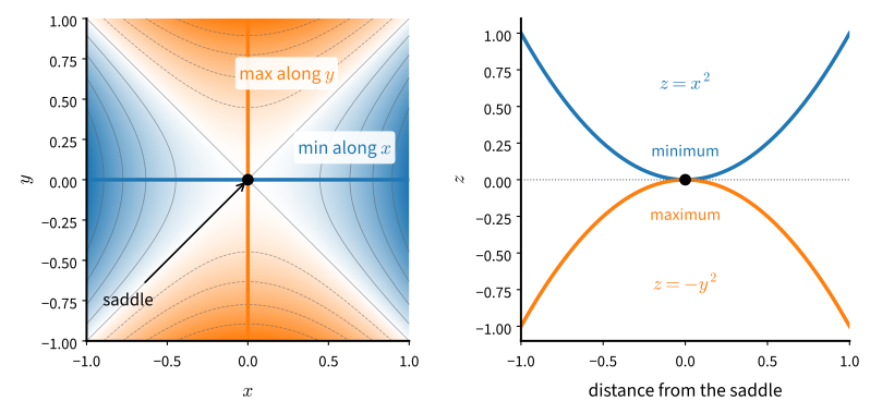
High-dim: a zero-gradient point is a minimum only if all Hessian eigenvalues are positive — with mixed signs it is a saddle. At 10^6 parameters, nearly every critical point is a saddle under the balanced-sign heuristic:
The origin is a minimum along one axis and a maximum along the other, giving a saddle with mixed Hessian signs.
Vanishing gradients
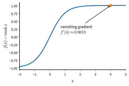
No critical point needed: f(x) = \tanh(x) at x = 4 has f'(4) \approx 0.0013. The surface is flat near the initial point:
At x=4, \tanh x has a very small gradient without a nearby critical point; flatness alone can stall descent.
ReLU and good initialization fixed this at the model level — not the optimizer’s job.
Effect of curvature
f(\mathbf{x}) = 0.1 x_1^2 + 2 x_2^2: curvatures 0.2 and 4, one learning rate. Steep direction caps \eta < 0.5; flat direction then keeps > 90\% of its value per step:
def f_valley(x1, x2): # Second derivatives 0.2 and 4return0.1* x1 **2+2* x2 **2def gd_valley(x1, x2, s1, s2): eta =0.45# Just under the stability ceiling of 0.5return (x1 - eta *0.2* x1, x2 - eta *4* x2, 0, 0)d2l.show_trace_2d(f_valley, d2l.train_2d(gd_valley, steps=30))
epoch 30, x1: -0.295265, x2: -0.002476
The iterate oscillates across the valley and advances slowly along it. Condition number \kappa =
\lambda_{\max}/\lambda_{\min} = 20; iterations scale linearly with \kappa. Real networks: \kappa in the thousands.
On strongly convex quadratics, momentum improves the condition-number dependence to \sqrt{\kappa}. Adam uses per-coordinate rescaling, and Muon uses per-matrix rescaling. Each method reduces the effect of anisotropic curvature.
Measured reality (Cohen et al., 2021): causality runs backwards — training raises sharpness (“progressive sharpening”) until it reaches \approx 2/\eta, then hovers there. Loss keeps falling, non-monotonically, in the “forbidden” regime.
The ceiling is an attractor, not a fence: pick \eta, the network adapts its curvature to it.
Training often lies outside the monotone-descent regime analyzed by the proofs.
One reason warmup and schedules matter (§ Schedules); measured on a 25-parameter net in the math appendix.
Effect of gradient noise
The gradient is a minibatch estimate: unbiased, variance \propto 1/b (measured on a real network in the SGD section).
Constant \eta → no convergence: a noise ball of squared radius \propto \eta. Hence decaying learning rates and schedules.
Batch size = a second dial, with hardware consequences (Minibatches) and diminishing returns at scale (Batch Size).
Momentum’s second job: averaging noise over time.
Noise can move the iterate away from saddles and shallow minima; deep barriers stay expensive.
The role of convexity
Deep losses are not convex — permutation symmetry alone gives every minimum d! separated copies; convex minima form one connected set.
Useful consequences include:
Language and baselines: condition number, rates, noise ball — all theorems for convex objectives. A method that fails on a quadratic is unlikely to succeed on a transformer.
Local approximation: near a good minimum the loss is approximately a quadratic bowl — which is why the valley cartoon predicts late-training behavior (and why weight averaging works).
Full treatment: the convexity chapter of the math appendix.
Recap
Minimizing training loss ≠ minimizing test loss; that gap belongs to regularization, not the optimizer.
Classical hazards: local minima, saddles (dominant in high dim), vanishing gradients.
Practical hazards: curvature (condition number \kappa) and noise (minibatch variance).
In modern networks, training often equilibrates at the edge of stability.
The toolkit ahead = three decisions: direction, step size over time, living with noise.