Gradient Descent

Deep networks are usually trained with SGD or its descendants rather than full-batch gradient descent. The simpler full-batch setting isolates their shared issues: LR sensitivity, divergence, local minima, poor conditioning, second-order corrections.

The rule:

x \leftarrow x - \eta \nabla f(x).

A first-order Taylor expansion shows that for sufficiently small \eta, this decreases f locally. Performance depends on the choice of \eta.

1D demo: f(x) = x^2

Setup and define f, f':

%matplotlib inline
from d2l import jax as d2l
import jax
from jax import numpy as jnp
import numpy as np

def f(x):  # Objective function
    return x ** 2

def f_grad(x):  # Gradient (derivative) of the objective function
    return 2 * x

GD iteration

Start at x = 10, \eta = 0.2, 10 steps. Converges to 0:

def gd(eta, f_grad):
    x = 10.0
    results = [x]
    for i in range(10):
        x -= eta * f_grad(x)
        results.append(float(x))
    print(f'epoch 10, x: {x:f}')
    return results

results = gd(0.2, f_grad)

epoch 10, x: 0.060466

def show_trace(results, f):
    n = max(abs(min(results)), abs(max(results)))
    f_line = d2l.arange(-n, n, 0.01)
    d2l.set_figsize()
    d2l.plot([f_line, results], [[f(x) for x in f_line], [
        f(x) for x in results]], 'x', 'f(x)', fmts=['-', '-o'])

show_trace(results, f)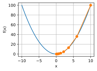

Learning rate too small

\eta = 0.05: takes forever to converge:

show_trace(gd(0.05, f_grad), f)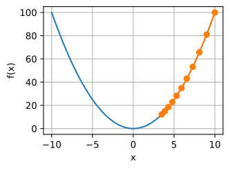

epoch 10, x: 3.486784

Learning rate too big

\eta = 1.1: the \mathcal{O}(\eta^2 f'^2) Taylor remainder dominates and the iterates diverge:

show_trace(gd(1.1, f_grad), f)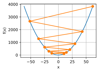

epoch 10, x: 61.917364

Gradient descent on a nonconvex objective

f(x) = x \cos(cx) has infinitely many local minima. Even with a moderately large learning rate, GD ends up in whichever basin it falls into:

c = d2l.tensor(0.15 * np.pi)

def f(x):  # Objective function
    return x * d2l.cos(c * x)

def f_grad(x):  # Gradient of the objective function
    return d2l.cos(c * x) - c * x * d2l.sin(c * x)

show_trace(gd(2, f_grad), f)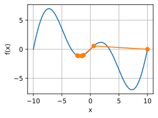

epoch 10, x: -1.528165

Multivariate GD

Same rule on vectors:

\mathbf{x} \leftarrow \mathbf{x} - \eta \nabla f(\mathbf{x}).

For f(x_1, x_2) = x_1^2 + 2 x_2^2, the x_2 direction has greater curvature.

def train_2d(trainer, steps=20, f_grad=None):
    """Optimize a 2D objective function with a customized trainer."""
    # `s1` and `s2` are internal state variables used by the stateful
    # optimizers (momentum, Adam) later in this chapter
    x1, x2, s1, s2 = -5, -2, 0, 0
    results = [(x1, x2)]
    for i in range(steps):
        if f_grad:
            x1, x2, s1, s2 = trainer(x1, x2, s1, s2, f_grad)
        else:
            x1, x2, s1, s2 = trainer(x1, x2, s1, s2)
        results.append((x1, x2))
    print(f'epoch {i + 1}, x1: {float(x1):f}, x2: {float(x2):f}')
    return results

def show_trace_2d(f, results):
    """Show the trace of 2D variables during optimization."""
    d2l.set_figsize()
    d2l.plt.plot(*zip(*results), '-o', color='#ff7f0e')
    x1, x2 = d2l.meshgrid(d2l.arange(-5.5, 1.0, 0.1),
                          d2l.arange(-3.0, 1.0, 0.1))
    d2l.plt.contour(x1, x2, f(x1, x2), colors='#1f77b4')
    d2l.plt.xlabel('x1')
    d2l.plt.ylabel('x2')

Multivariate trajectory

def f_2d(x1, x2):  # Objective function
    return x1 ** 2 + 2 * x2 ** 2

def f_2d_grad(x1, x2):  # Gradient of the objective function
    return (2 * x1, 4 * x2)

def gd_2d(x1, x2, s1, s2, f_grad):
    g1, g2 = f_grad(x1, x2)
    return (x1 - eta * g1, x2 - eta * g2, 0, 0)

eta = 0.1
show_trace_2d(f_2d, train_2d(gd_2d, f_grad=f_2d_grad))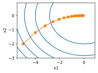

epoch 20, x1: -0.057646, x2: -0.000073

The path bends: the two coordinates want different step sizes. One global \eta can’t satisfy both.

Newton’s method: second-order

Use the Hessian to set the step size automatically. From the second-order Taylor expansion:

\mathbf{x} \leftarrow \mathbf{x} - [\nabla^2 f(\mathbf{x})]^{-1} \nabla f(\mathbf{x}).

For f(x) = \cosh(cx), a few Newton steps reach the minimum without a manually chosen learning rate:

c = d2l.tensor(0.5)

def f(x):  # Objective function
    return d2l.cosh(c * x)

def f_grad(x):  # Gradient of the objective function
    return c * d2l.sinh(c * x)

def f_hess(x):  # Hessian of the objective function
    return c**2 * d2l.cosh(c * x)

def newton(eta=1):
    x = 10.0
    results = [x]
    for i in range(10):
        x -= eta * f_grad(x) / f_hess(x)
        results.append(float(x))
    print(f'epoch 10, x: {float(x):f}')
    return results

show_trace(newton(), f)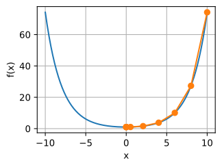

epoch 10, x: 0.000000

Newton’s method under negative curvature

f(x) = x \cos(cx): Newton divides by the second derivative, so negative curvature sends it uphill, toward a maximum. Damping (\eta = 0.5) restores sanity:

c = d2l.tensor(0.15 * np.pi)

def f(x):  # Objective function
    return x * d2l.cos(c * x)

def f_grad(x):  # Gradient of the objective function
    return d2l.cos(c * x) - c * x * d2l.sin(c * x)

def f_hess(x):  # Hessian of the objective function
    return - 2 * c * d2l.sin(c * x) - x * c**2 * d2l.cos(c * x)

show_trace(newton(), f)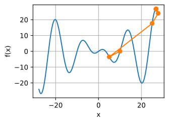

epoch 10, x: 26.834133

show_trace(newton(0.5), f)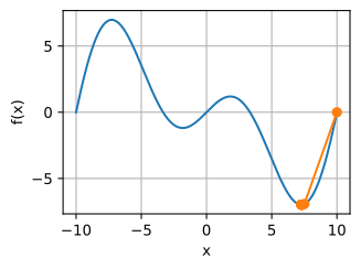

epoch 10, x: 7.269860

Approximate preconditioning

Full Newton at d \sim 10^9: \mathcal{O}(d^2) memory, an \mathcal{O}(d^3) solve. Storing the Hessian alone would require exabytes.

Deep-learning optimizers instead rescale updates with inexpensive approximations to curvature.

\mathbf{x} \leftarrow \mathbf{x} - \eta\, \textrm{diag}(\mathbf{H})^{-1} \nabla f(\mathbf{x})

= a separate learning rate per coordinate (fixes the millimeters-vs-kilometers mismatch automatically).

Diagonal preconditioners estimated from gradients → AdaGrad, Adam. Per-matrix preconditioning → Muon. Both later in this chapter.

Recap

GD update: x \leftarrow x - \eta \nabla f(x).
Learning rate too small → slow; too large → diverge.
Local minima trap plain GD on non-convex objectives.
Newton uses the Hessian as the ideal preconditioner — one step on quadratics, but \mathcal{O}(d^2) memory and unsafe under negative curvature.
Deep-learning methods use inexpensive preconditioning: per-coordinate (Adam) and per-matrix (Muon) rescaling.