Implementation of Multilayer Perceptrons

Dive into Deep Learning · §4.2

Implementing a Multilayer Perceptron
From-scratch and framework-layer implementations; the displayed run reaches \approx 0.87 validation accuracy

The MLP architecture

What we are building

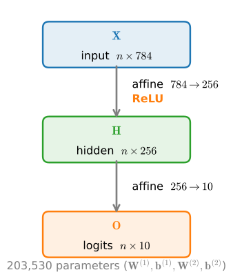
A batched image is flattened to 784 features, mapped by an affine layer + ReLU to a 256-dim hidden vector, then by a second affine layer to 10 logits.

  • One hidden layer, one nonlinearity.
  • Same loss, loaders, and Trainer as softmax regression.

That ReLU between the two affine maps, together with the hidden layer, is the entire difference from a linear classifier like softmax regression.
Why these sizes?

Design choices

Fashion-MNIST: 784 inputs, 10 classes. We pick 256 hidden units, giving \approx 200\text{k} parameters.

  • Width 256: a representative capacity for this example.
  • A power of 2: often favorable for accelerator kernels, although performance depends on hardware and precision.
  • One hidden layer suffices here; spatial structure waits for convolutions.

Depth, width, and learning rate are hyperparameters: chosen by hand, not learned.

01

From Scratch

parameters, ReLU, and forward by hand

Parameters: two weights, two biases

From Scratch

class MLPScratch(d2l.Classifier):
    def __init__(self, num_inputs, num_outputs, num_hiddens, lr,
                 sigma=0.01, rngs=None):
        super().__init__()
        self.save_hyperparameters(ignore=['rngs'])
        rngs = nnx.Rngs(d2l.get_key()) if rngs is None else rngs
        self.W1 = nnx.Param(
            rngs.params.normal((num_inputs, num_hiddens)) * sigma)
        self.b1 = nnx.Param(jnp.zeros(num_hiddens))
        self.W2 = nnx.Param(
            rngs.params.normal((num_hiddens, num_outputs)) * sigma)
        self.b2 = nnx.Param(jnp.zeros(num_outputs))

Weights start as small Gaussian noise (\sigma=0.01) to break symmetry, biases at zero:

\mathbf{W}^{(1)}\!\in\mathbb{R}^{784\times256},\; \mathbf{b}^{(1)}\!\in\mathbb{R}^{256} \mathbf{W}^{(2)}\!\in\mathbb{R}^{256\times10},\; \mathbf{b}^{(2)}\!\in\mathbb{R}^{10}

784\cdot256 + 256 + 256\cdot10 + 10 = 203{,}530 learnable numbers.

ReLU, by hand

From Scratch

We write the activation directly as \max(x, 0), applied elementwise:

def relu(X):
    return jnp.maximum(X, 0)

Map negative inputs to zero and retain positive inputs. This nonlinearity prevents the affine maps from collapsing into one.

The forward pass is two lines

From Scratch

Flatten, then an affine-ReLU, then a second affine, exactly the data flow in the diagram:

\mathbf{H} = \mathrm{ReLU}(\mathbf{X}\mathbf{W}^{(1)} + \mathbf{b}^{(1)}), \qquad \mathbf{O} = \mathbf{H}\mathbf{W}^{(2)} + \mathbf{b}^{(2)}.

def forward(self, X):
    X = d2l.reshape(X, (-1, self.num_inputs))
    H = relu(d2l.matmul(X, self.W1) + self.b1)
    return d2l.matmul(H, self.W2) + self.b2

Training the from-scratch model

From Scratch

The loss, the loaders, and the Trainer are unchanged from softmax regression. Only the model class is new:

In this run, validation accuracy settles around \approx 0.87 over 30 epochs, a modest gain over the softmax regression baseline on the same data, for a model with one hidden layer and a ReLU.

02

Concise

framework layers register parameters and compose operations

The same model, declared

Concise

NNX stores each layer as an ordinary attribute and registers its parameters automatically:

class MLP(d2l.Classifier):
    def __init__(self, num_outputs, num_hiddens, lr, num_inputs=784,
                 rngs=None):
        super().__init__()
        self.save_hyperparameters(ignore=['rngs'])
        rngs = nnx.Rngs(d2l.get_key()) if rngs is None else rngs
        self.hidden = nnx.Linear(num_inputs, num_hiddens, rngs=rngs)
        self.output = nnx.Linear(num_hiddens, num_outputs, rngs=rngs)

    def forward(self, X):
        X = X.reshape((X.shape[0], -1))  # Flatten
        return self.output(nnx.relu(self.hidden(X)))

No hand-written parameter dictionary: each nnx.Linear owns its weights from construction onward.

Same architecture as the diagram, one compact method.

Reusing the training loop

Concise

The concise model reuses the same trainer and data. Its trajectory can differ because its initializer is different:

model = MLP(num_outputs=10, num_hiddens=256, lr=0.1)
trainer.fit(model, data)

Same architecture, different init (framework default vs \mathcal{N}(0, 0.01^2)), so trajectories differ slightly.

03

What’s next

from a working MLP to a reliable one

Four open questions

Where this goes

We have a working MLP. Making it reliable is the rest of this chapter:

  • Backprop (the forward/backward-propagation section): how gradients flow through an arbitrary stack.
  • Initialization (the numerical-stability section): choose \sigma so signals neither vanish nor explode through depth.
  • Generalization (the generalization-in-deep-learning section): why a flexible model does well on unseen data at all.
  • Regularization (the dropout section): dropout, and friends.

Each question gets its own section, and exercise 2 hands you the next question: add a second hidden layer while keeping \sigma = 0.01, and the deeper net trains worse. The numerical-stability section explains.

Recap

Wrap-up

  • An MLP = a linear classifier plus a hidden layer and a nonlinearity between affine maps.
  • From scratch: four parameter tensors, a hand-rolled ReLU, a two-line forward. Concrete, but tedious to ship.
  • Concise: declare the layer stack; Sequential holds the parameters and defines the forward pass.
  • Both forms declare the same architecture (inits differ).
  • The training loop is unchanged from softmax regression (modularity paying off).
  • Hyperparameters (depth, width, lr) live outside the model; the same loop trains any of them.
  • The displayed run settles around \approx 0.87; a controlled comparison would also match seeds, initialization, and optimization settings.

The next section derives the gradients computed by backward() and verifies them numerically.