Singular Value Decomposition and Low-Rank Approximation

Dive into Deep Learning · §24.3

The SVD, Eckart–Young, and Low-Rank Approximation

The SVD for General Matrices

Motivation

Eigendecomposition requires a square matrix, and a defective matrix has no eigenbasis.

The singular value decomposition gives a rotate–scale–rotate factorization for every matrix, including rectangular and defective matrices.

The factorization determines rank, low-rank approximations, PCA, the pseudoinverse, and the condition number.

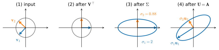
A general \mathbf{A} bends the unit circle to an ellipse; the SVD names the two frames that do it.

The factorization

rotate, scale, rotate

Rotate–scale–rotate

The factorization

Every m\times n matrix factors as \mathbf{A}=\mathbf{U}\boldsymbol{\Sigma}\mathbf{V}^\top (\mathbf{U},\mathbf{V} orthogonal, \sigma_1\ge\cdots\ge0). Reading right to left, \mathbf{V}^\top rotates, \boldsymbol{\Sigma} scales by \sigma_i, \mathbf{U} rotates, one stretch \mathbf{A}\mathbf{v}_i=\sigma_i\mathbf{u}_i:

The top one is the Rayleigh quotient again: \sigma_1=\max_{\|\mathbf{x}\|=1}\|\mathbf{A}\mathbf{x}\|=\|\mathbf{A}\|_2, the most \mathbf{A} can stretch any unit vector (its spectral norm).

Where the singular values come from

The factorization

The SVD is the spectral theorem applied to \mathbf{A}^\top\mathbf{A}.

(1) \mathbf{A}^\top\mathbf{A} is symmetric and PSD (\mathbf{x}^\top\mathbf{A}^\top\mathbf{A}\mathbf{x}=\|\mathbf{A}\mathbf{x}\|^2\ge0), so it has an orthonormal eigenbasis \mathbf{v}_i with eigenvalues \lambda_i\ge0.

(2) Take square roots and apply \mathbf{A}: \;\sigma_i=\sqrt{\lambda_i}, \;\mathbf{u}_i=\mathbf{A}\mathbf{v}_i/\sigma_i.

(3) The output frame is orthonormal by construction: \mathbf{u}_i^\top\mathbf{u}_j=\sigma_i^{-1}\sigma_j^{-1}\, \mathbf{v}_i^\top\mathbf{A}^\top\mathbf{A}\,\mathbf{v}_j=\delta_{ij}.

Gram matrices are never defective, so the SVD never fails, for any matrix, rectangular or defective.

SVD of a Defective Shear

The factorization

The shear \begin{bmatrix}1&1\\0&1\end{bmatrix} is defective: one eigenvalue \lambda=1, only a one-dimensional eigenspace, no eigenbasis.

Its SVD has no such trouble: the singular values are the golden ratio and its reciprocal (\sigma_1\sigma_2=|\det\mathbf{A}|=1):

singular values of the shear: [1.618034 0.618034]
golden ratio phi, 1/phi:     [1.618034 0.618034]
product sigma_1 * sigma_2 = |det A| = 1.0

Left and Right Singular Vectors

The factorization

The action \mathbf{A}\mathbf{v}_i=\sigma_i\mathbf{u}_i verifies in one line: reconstruction is exact, and the squared singular values are the eigenvalues of \mathbf{A}^\top\mathbf{A}.

A = np.array([[3., 1.], [1., 3.], [0., 2.]])   # a 3x2 matrix
U, s, Vt = np.linalg.svd(A, full_matrices=False)
recon = (U * s) @ Vt
eig = np.sort(np.linalg.eigvalsh(A.T @ A))[::-1]
print('reconstruction error:', round(float(np.linalg.norm(recon - A)), 12))
print('sigma^2          :', (s ** 2).round(6))
print('eig(A^T A) sorted:', eig.round(6))

reconstruction error: 0.0
sigma^2          : [18.324555  5.675445]
eig(A^T A) sorted: [18.324555  5.675445]

A ranked sum of rank-one pieces

The factorization

Column by column, \mathbf{A}=\mathbf{U}\boldsymbol{\Sigma}\mathbf{V}^\top unrolls into dyads, heaviest first:

\mathbf{A} = \sum_{i=1}^{r} \sigma_i\,\mathbf{u}_i\mathbf{v}_i^\top.

In Einstein notation that sum is the index pattern 'i,mi,in->mn', and the one-liner rebuilds the matrix exactly:

rng = np.random.default_rng(5)
A = rng.standard_normal((4, 3))
U, s, Vt = np.linalg.svd(A, full_matrices=False)   # thin SVD
A_dyads = np.einsum('i,mi,in->mn', s, U, Vt)       # sum_i sigma_i u_i v_i^T
print('dyadic rebuild error:', round(float(np.linalg.norm(A_dyads - A)), 12))

dyadic rebuild error: 0.0

Low-rank approximation truncates this ordered list of rank-one terms by retaining the leading terms and discarding the smaller ones.

Rank & the four fundamental subspaces

The factorization

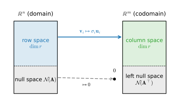
\operatorname{rank}\mathbf{A} is the number of nonzero \sigma_i. The singular vectors split into the row/null space (input) and column/left-null space (output); \mathbf{A} is a bijection between the row and column spaces.

In floating point, threshold tiny \sigma_i: numerical rank counts \sigma_i>\sigma_1\max(m,n)\,\epsilon_{\text{mach}}.

\mathbf{A} maps the row space onto the column space and maps the null space to zero.

Numerical rank in practice

The factorization

A deliberately rank-2 matrix in \mathbb{R}^{4\times4}: two singular values collapse to machine zero, so a tolerance recovers the true rank where a test for exact zeros would fail.

rng = np.random.default_rng(0)
A = rng.standard_normal((4, 2)) @ rng.standard_normal((2, 4))  # rank <= 2
s = np.linalg.svd(A, compute_uv=False)
print('singular values:', s.round(6))
print('numerical rank :', int(np.linalg.matrix_rank(A)))

singular values: [4.351705 0.914865 0.       0.      ]
numerical rank : 2

Low-rank approximation

retain the leading terms, discard the smaller ones

Eckart–Young: optimal low rank

Approximation

Keep the top k dyads, \mathbf{A}_k=\sum_{i\le k}\sigma_i\mathbf{u}_i\mathbf{v}_i^\top.

\mathbf{A}_k is the provably best rank-k approximation: \|\mathbf{A}-\mathbf{A}_k\|_2=\sigma_{k+1}, and \|\cdot\|_F^2=\sum_{i>k}\sigma_i^2 (the case PCA uses).

Why no rank-k \mathbf{B} does better, by dimension counting: \dim\ker\mathbf{B}\ge n-k, and \mathcal{V}=\operatorname{span}\{\mathbf{v}_1,\dots,\mathbf{v}_{k+1}\} has dim k+1.

Their dimensions exceed that of \mathbb{R}^n: (n-k)+(k+1)>n, so a unit \mathbf{x} belongs to both, with \mathbf{B}\mathbf{x}=\mathbf 0.

There \mathbf{B} vanishes while \mathbf{A} still stretches the vector: \|(\mathbf{A}-\mathbf{B})\mathbf{x}\|=\|\mathbf{A}\mathbf{x}\|\ge\sigma_{k+1}. The energy ratio \sum_{i\le k}\sigma_i^2/\sum_i\sigma_i^2 determines the compression–error tradeoff.

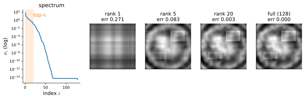
Image truncation illustrates the Eckart–Young error

Approximation

The spectrum decays rapidly (log scale, left), so the rank-20 approximation has low visible error while storing a fraction of the entries; the discarded \sigma_i carry little energy.

Singular-value spectrum and rank-k reconstructions, each labeled with its relative Frobenius error.

PCA = Eckart–Young on centered data

Approximation

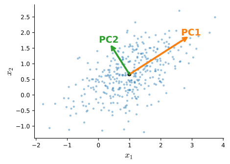
Center the data, then the top right singular vectors \mathbf{v}_i are the principal directions; component i explains variance \sigma_i^2/n. The SVD axes and the covariance eigenvalues agree exactly:

explained variance (sigma^2/n): [8.0873 0.5705]
eigenvalues of covariance     : [8.0873 0.5705]
explained-variance ratio      : [0.9341 0.0659]

Principal axes scaled by \sigma_i/\sqrt{n}; the first aligns with the direction of maximal variance.

Solving & conditioning

the pseudoinverse and condition number

Pseudoinverse & least squares

Solving

Invert the nonzero singular values and transpose the rotations, \mathbf{A}^{+}=\mathbf{V}\boldsymbol{\Sigma}^{+}\mathbf{U}^\top. The SVD basis decouples the problem, so \mathbf{A}^{+}\mathbf{b} is the minimum-norm least-squares solution. pinv and lstsq agree, and forming \mathbf{A}^\top\mathbf{A} squares the conditioning:

pinv : [3.5 1.4]  residual 2.0494
lstsq: [3.5 1.4]  residual 2.0494
cond(A)     = 7.469
cond(A^T A) = 55.782 = cond(A)^2

The condition number

Solving

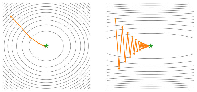
\kappa(\mathbf{A})=\sigma_1/\sigma_r is one number, two consequences: it bounds error amplification in a solve and the gradient-descent contraction (\kappa-1)/(\kappa+1) on a quadratic bowl.

Forming \mathbf{A}^\top\mathbf{A} squares it, \kappa(\mathbf{A}^\top\mathbf{A})=\kappa(\mathbf{A})^2, which is why the normal equations are numerically worse.

Well-conditioned bowl (near-circular, a straight path) versus ill-conditioned (elongated, a zig-zag).

In modern deep learning

low rank is everywhere

The SVD in modern deep learning

Applications

LoRA learns a rank-r correction \Delta\mathbf{W}=\mathbf{B}\mathbf{A} at r(m+n) params; Eckart–Young bounds how well any rank-r update can track the full one (\sigma_{r+1}).
Spectral norm caps \sigma_1=\|\mathbf{W}\|_2 for Lipschitz control, estimated by power iteration on \mathbf{W}^\top\mathbf{W}.

Muon even optimizes through the SVD, stepping along the polar factor \mathbf{U}\mathbf{V}^\top of the momentum (Newton–Schulz, matmuls only).

Newton–Schulz Iteration in Muon

Applications

Newton–Schulz, \mathbf{X}\leftarrow\tfrac12(3\mathbf{X}-\mathbf{X}\mathbf{X}^\top\mathbf{X}), applies the odd cubic p(\sigma)=\tfrac12(3\sigma-\sigma^3) to every singular value while leaving \mathbf{U} and \mathbf{V} untouched; Frobenius normalization first puts every \sigma inside the cubic’s basin of attraction of 1. The following output shows the spectrum across iterations:

iter  2: sigma = [0.9982 0.8554 0.4648 0.1499]
iter  4: sigma = [1.     0.9987 0.8351 0.3291]
iter  6: sigma = [1.     1.     0.9978 0.6599]
iter  8: sigma = [1.     1.     1.     0.9663]
iter 10: sigma = [1. 1. 1. 1.]
distance to polar factor U V^T: 4e-06

Every \sigma_i \to 1; the smallest converges slowest, which is the regime Muon’s tuned coefficients accelerate. The iterate converges to the polar factor \mathbf{U}\mathbf{V}^\top using matrix multiplications without computing an SVD.

Effective rank, measured

Applications

How small a rank suffices depends entirely on how fast the spectrum decays, so measure it. Here rank 18 of 256 holds 95% of the spectral energy, a LoRA at 10.5% of the parameters:

rng = np.random.default_rng(2)
m, n = 256, 512
sigma = np.exp(-np.arange(min(m, n)) / 12.0)                 # fast-decaying spectrum
Uw, _ = np.linalg.qr(rng.standard_normal((m, min(m, n))))
Vw, _ = np.linalg.qr(rng.standard_normal((n, min(m, n))))
s = np.linalg.svd((Uw * sigma) @ Vw.T, compute_uv=False)
r95 = int(np.searchsorted(np.cumsum(s ** 2) / (s ** 2).sum(), 0.95) + 1)
print(f'{m} x {n} matrix; rank for 95% energy: {r95}; '
      f'LoRA params {r95 * (m + n) / (m * n):.1%} of full')

256 x 512 matrix; rank for 95% energy: 18; LoRA params 10.5% of full

The yardstick is the Marchenko–Pastur bulk of the previous section: trained weight spectra are heavy-tailed far beyond that noise baseline, and the escapees are the learned correlation.

Two orthonormal bases expose rank and approximation

Wrap-up

Rotate, scale, rotate: \mathbf{A}=\mathbf{U}\boldsymbol{\Sigma}\mathbf{V}^\top, \sigma_i=\sqrt{\lambda_i(\mathbf{A}^\top\mathbf{A})}, never fails.
Eckart–Young: top-k truncation is the optimal low-rank approximation; the energy ratio measures the retained spectral energy.
PCA is Eckart–Young on centered data.

Pseudoinverse \mathbf{A}^{+} gives min-norm least squares.
\kappa=\sigma_1/\sigma_r summarizes conditioning; the normal equations square it.
Powers PCA, LoRA, Muon, and spectral normalization.

Rank, range, approximation, PCA, and conditioning: all from one factorization.